Hands-on decision models
Visual guide to Jev-like models
How Jev and its open reproductions turn small language models into functions that return typed, calibrated answers instead of text
Chapter 1
What do we need decision models for?
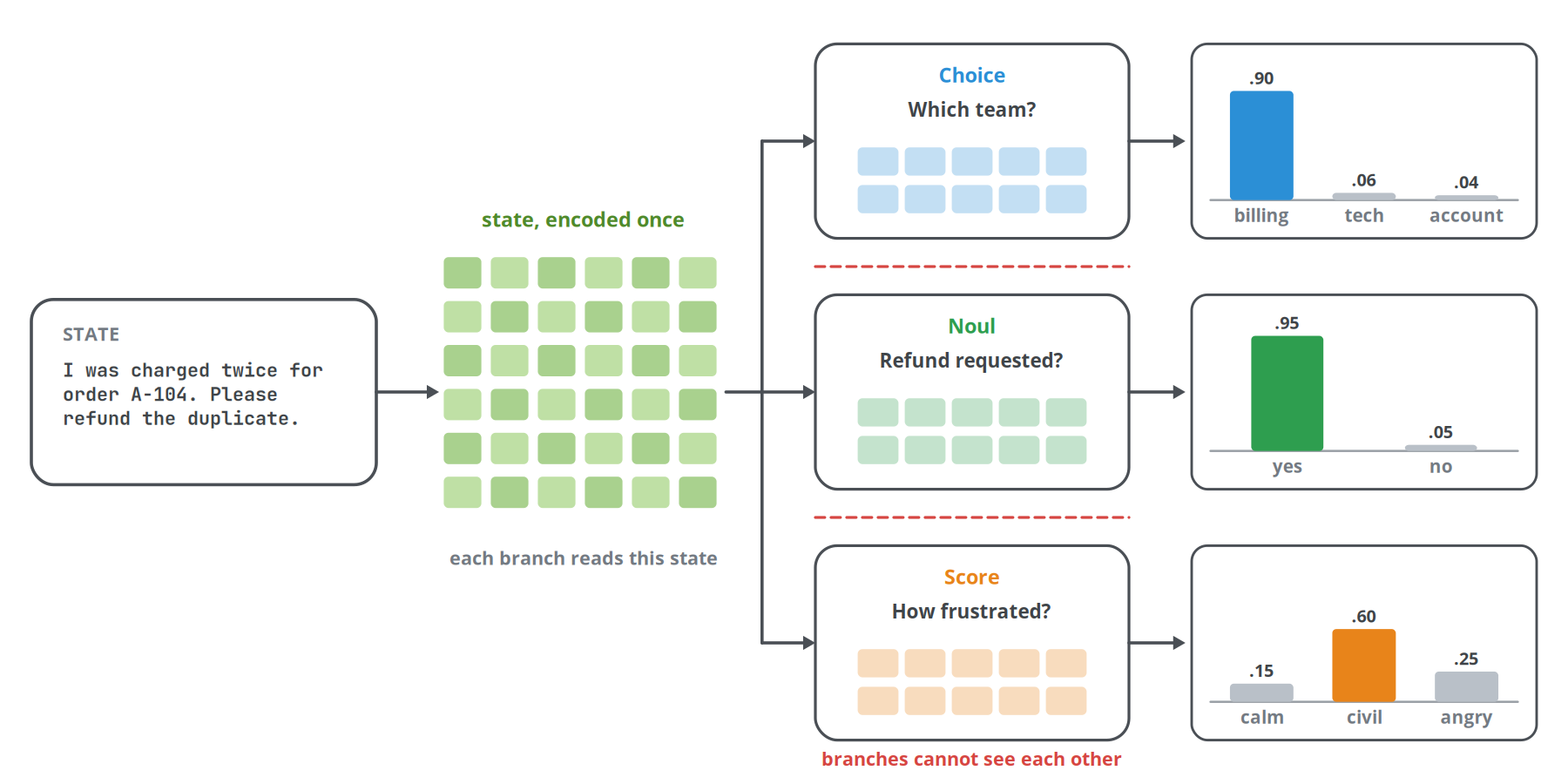
Let's imagine that a support ticket arrives at 9:14 on a Monday. Before anyone replies, software has to answer several small questions about it.
The ticket reads:
Support ticketHi, I was charged twice for order A-104. Please refund the duplicate today or I will cancel my plan.
This ticket will be the reference example of the book. With today's popular approach, this could be handled by a generative LLM agent. An agent that handles it has to check that the message is safe to process, pick the team that owns it, notice that the customer asks for a refund and threatens to leave, estimate how frustrated they are, choose a tool, and decide whether a person should approve the refund before money moves. However, only one of these steps, writing the reply, is generative. For every other step, the problem you are actually trying to solve is classification, in other words a decision.
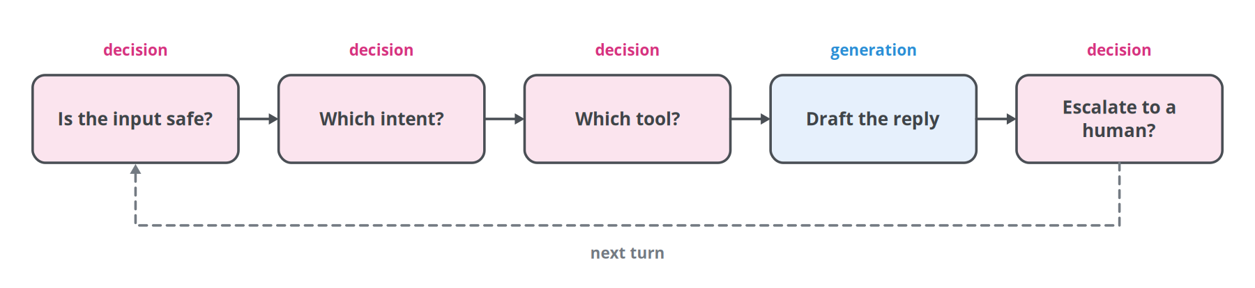
A decision is a question whose valid answers are fixed before the call: a set of labels, an ordered scale, or yes and no. Replies, summaries and code are generation.
Despite that, most teams answer decisions with the same chat model that writes replies. The prompt describes the question and the allowed labels. The model writes a JSON object, the application parses it, validates it against a schema and retries when validation fails. The approach works, but it is very inefficient, and it has two costs that grow with traffic.
The first cost is time. A decoder produces output one token at a time, and each token needs a full pass through the network. Even a tiny answer such as {"team": "billing"} takes about eight passes, and a reasoning model may spend thousands of tokens before it writes the answer.
The second cost is meaning. If you ask the model for a confidence, it writes something like "confidence": 0.9. That number, however, is not tied to how likely the answer is to be correct. No part of training connected it to how often the model is right, and post-training for chat makes the model's internal probabilities worse calibrated than those of the pretrained model it started from; the GPT-4 technical report shows this on a multiple-choice benchmark [47]. An application cannot build a policy on a number with no known relation to accuracy.
How much time can we save?
SemIf, one of the first open projects in this area, measured the time cost on one RTX 3090 [11]. The same frozen Qwen3.5-4B read the same state and answered 21 yes/no questions in two ways. Generating the shortest possible JSON array, 21 bare "yes" and "no" values without keys, took 5.33 s and 111 output tokens. Reading the answers directly from the model's output layer took 1.02 s and produced no tokens at all.
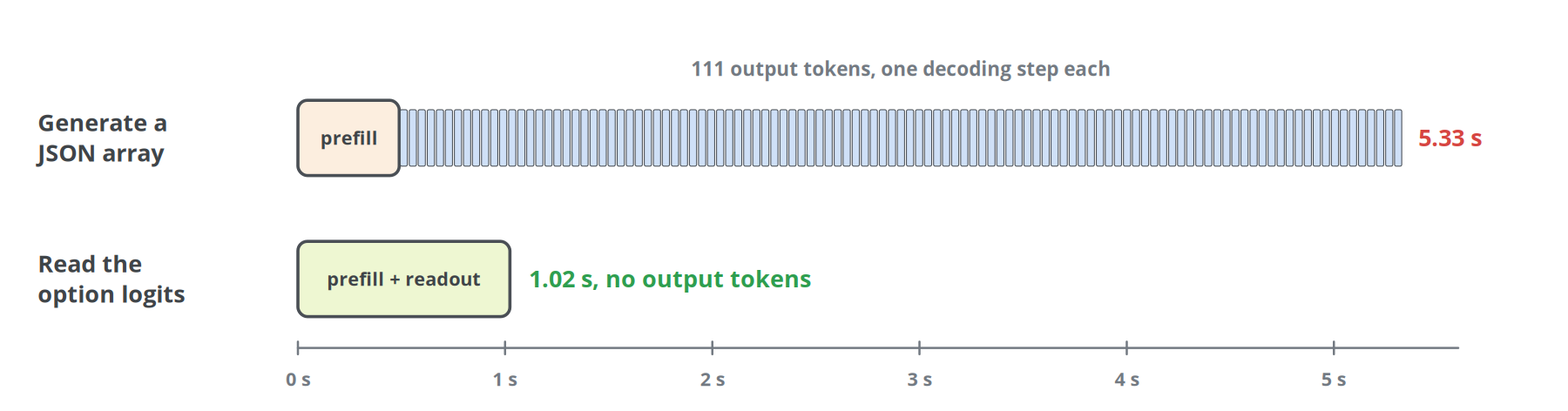
The two paths agreed on 18 of the 21 answers, so they are close but not identical. The speed difference has a simple cause. Processing the prompt, called prefill, handles all input tokens in parallel. After prefill, the information needed to choose between "yes" and "no" is already present in the network's hidden state at the last position. Generation spends the remaining time writing that information out one token at a time.
What a decision model changes
A decision model skips the writing. It reads the ticket once, reads the questions, and returns for each question a probability for every allowed answer. The application receives numbers it can compare against thresholds, and there is no text to parse.
TypeSafe AI released what is probably the first commercial model of this kind, Jev, on 15 September 2026, and named the category System One models after Kahneman's term for fast, intuitive judgment [1][43]. Within ten days, open projects had reproduced the interface with models from 340 million to 27 billion parameters [22].
The fastest way to understand these models is to start from something familiar. Chapter 2 explains how a fine-tuned text classifier works, and Chapter 3 changes one assumption at a time until it becomes a decision model.
Chapter 2
How a transformer classifier works
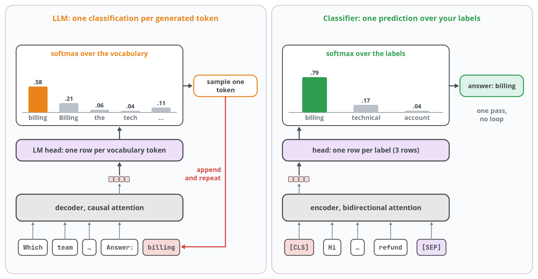
If most of your experience is with large language models, you already know more about classifiers than it may seem. An LLM writes text one token at a time. At each step it reads everything written so far and ends with one vector for the last position. That vector is multiplied by a large matrix with one row for every token in the vocabulary, typically 100,000 to 250,000 rows, which gives one score per token. These scores are the logits, and a softmax turns them into the next-token probabilities that an API reports as log-probabilities. The sampler then picks one token, appends it to the text and runs the model again.
Each of those steps is a classification: the input is the text so far, and the classes are the tokens of the vocabulary. Generation repeats that classification many times and feeds every answer back in as input.
A dedicated text classifier makes the same kind of prediction once, over a handful of classes that you choose. The question changes from "which token comes next?" to "which team should handle this ticket?". The large vocabulary matrix is replaced by a small one with one row per label, and there is no sampling loop: the most probable label is the answer, and its probability says how sure the model is.
Most of the vocabulary of LLM work carries over to classifiers, sometimes with a shifted meaning.
| In LLM work | In a text classifier |
|---|---|
| Prompt | The input text. There are no instructions, because the task is fixed in the weights |
| Tokens and tokenizer | The same idea: the input is split into tokens from a fixed vocabulary |
| Context window | The maximum input length, 512 tokens for BERT-era encoders |
| Next-token logits and log-probabilities | Logits and probabilities of the labels |
| Temperature | The same softmax temperature, used to calibrate probabilities, not to vary the output |
| Fine-tuning on example conversations | Fine-tuning on labelled examples, with a cross-entropy loss over the labels |
| Decoder-only model: GPT, Llama, Qwen | Usually an encoder from the BERT family, which reads the whole text in both directions |
The last row needs a word of explanation. The LLMs you use are decoders: each token may look only at the tokens before it, because a model that generates text left to right cannot look at words it has not written yet. A classifier generates nothing, so it can let every token look at the whole input, before and after it. A network built this way is called an encoder. The section on the encoder below shows the difference in attention masks.
Why train a classifier at all, when a chat model can be prompted to answer "billing", "technical" or "account"? Prompting needs no training data, and Chapter 4 shows how to read the answer from the token probabilities. A fine-tuned classifier has other advantages. BERT-base has 110 million parameters, less than a fiftieth of a 7-billion-parameter chat model, so it is far cheaper and faster per request and runs on a CPU. It also learns your labels from your examples, so its probabilities come from training on the task. The price is rigidity: the labels live in the weights, and a new label means new data and a new training run. The decision models in the rest of this book try to keep the shape of the classifier and the flexibility of the LLM.
The rest of this chapter opens the classifier up, part by part.
Put formally, a text classifier is a function that takes a piece of text and returns a probability distribution over a fixed set of labels. For the running example, the labels are the three teams that can own a ticket: billing, technical and account. The ticket goes in, and three probabilities that sum to one come out. Everything in this chapter explains how a transformer computes those three numbers and how it learns to compute them well.
Training: fine-tuning a pretrained encoder
Nobody trains a text classifier from random weights. The encoder is first pretrained on a large unlabelled corpus with a self-supervised task. BERT hides 15% of the input tokens and learns to predict them from both sides, which forces it to learn grammar, word meaning and a good deal of world knowledge [62]. Fine-tuning then adds the head, with random weights, and trains the whole network on labelled examples, here a few thousand tickets with their teams.
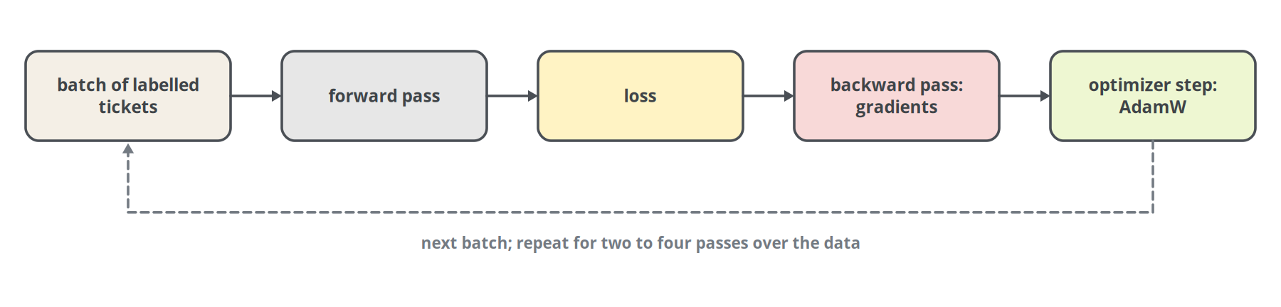
Each step takes a batch of examples, runs the forward pass, computes the average loss, computes gradients by backpropagation and lets the optimizer update the weights. The usual optimizer is AdamW, which adapts the step size for each parameter and applies weight decay separately from the gradient update [63]. The BERT authors recommend a learning rate between 2 × 10⁻⁵ and 5 × 10⁻⁵, a batch size of 16 or 32 and two to four passes over the data [62]. The learning rate usually rises linearly over the first steps and then falls to zero, so that the random head does not disturb the pretrained encoder with large early updates.
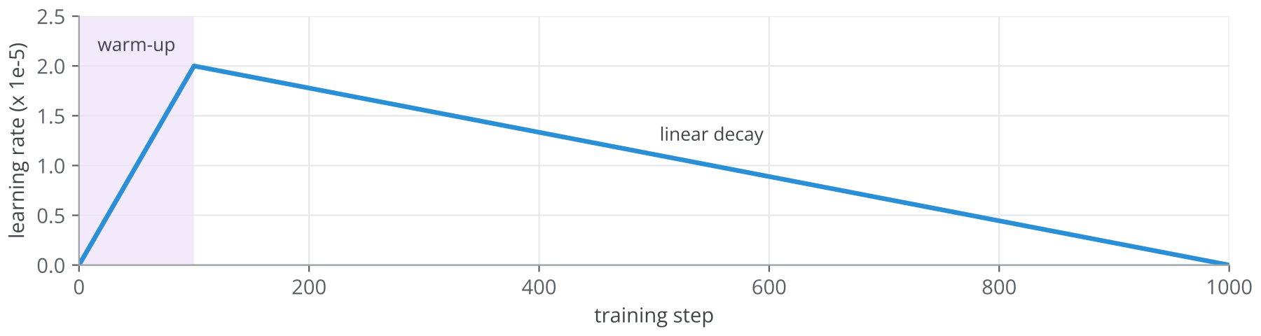
Fine-tuning on small datasets can be unstable: the same recipe with different random seeds can produce very different models. Mosbach and colleagues traced this to optimization problems early in training and recommend small learning rates, bias correction in Adam and more training steps [66]. A separate validation set guides the choice of learning rate and the number of epochs, and the test set stays untouched until the end.
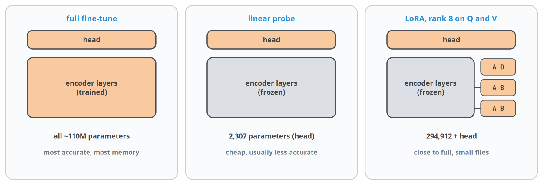
Three variants differ in which weights are trained. Full fine-tuning updates everything. A linear probe freezes the encoder and trains only the head, which is fast and cheap but usually less accurate. Low-rank adaptation, LoRA, freezes the original weights and trains small low-rank matrices added to some of them [42]. With rank 8 on the query and value maps of BERT-base, that is 294,912 trainable parameters, about 0.27% of the model. Many of the open decision models in this book are LoRA fine-tunes.
One label or several
Softmax with cross-entropy assumes that exactly one label is correct. A ticket belongs to one team, so routing fits. Other questions allow several labels at once: our ticket asks for a refund and threatens cancellation, and a third flag for a legal threat would be false. For that case the head produces one logit per label, each passes through its own sigmoid to a probability between zero and one, and the loss is a binary cross-entropy per label. The probabilities no longer sum to one, and each label gets its own threshold.
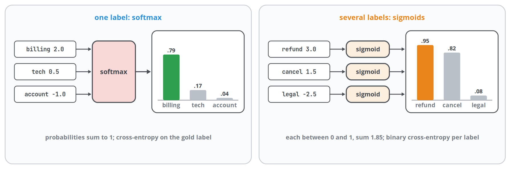
Mixing the two causes problems. A head trained with independent sigmoids and read at inference with a softmax across labels produces probabilities that the training never targeted. turlockmike suspected exactly this mismatch behind the overconfident scores of GLiNER2.5-Decide [24].
Imbalanced labels and evaluation
Real label distributions are rarely balanced. If 70% of tickets go to billing, a model that always answers billing reaches 70% accuracy and is useless. Per-label precision and recall show the problem, and their harmonic mean, F1, summarizes each label. Macro-averaged F1 gives every label equal weight; micro-averaged F1 weights labels by frequency and stays close to accuracy for single-label tasks. A confusion matrix, which counts how often each true label was predicted as each other label, shows which teams the model mixes up. Common remedies for imbalance are class weights in the loss, resampling the training data and choosing thresholds per label on validation data.
Why the probabilities come out overconfident
Cross-entropy keeps rewarding larger logits for the correct label as long as its probability is below one. A large network can push the training loss close to zero, and on new data its probabilities then come out higher than its accuracy justifies. Guo and colleagues measured this for modern networks and found that a single temperature fitted on held-out data corrects most of it [33]. Label smoothing attacks the same problem during training: the target is softened from 1 for the correct label and 0 for the others to, with a smoothing factor of 0.1 and three labels, 0.933 and 0.033 [64]. It tends to improve calibration, at some cost to how much information the logits keep about similar classes [65]. The chapter on calibration covers how to measure the result.
Chapter 3
From classifiers to decision models
The classifier described in the previous chapter is already good at classification, but it cannot change the question without retraining.
Below, we show how to move step by step from a fixed classifier to an increasingly general model.
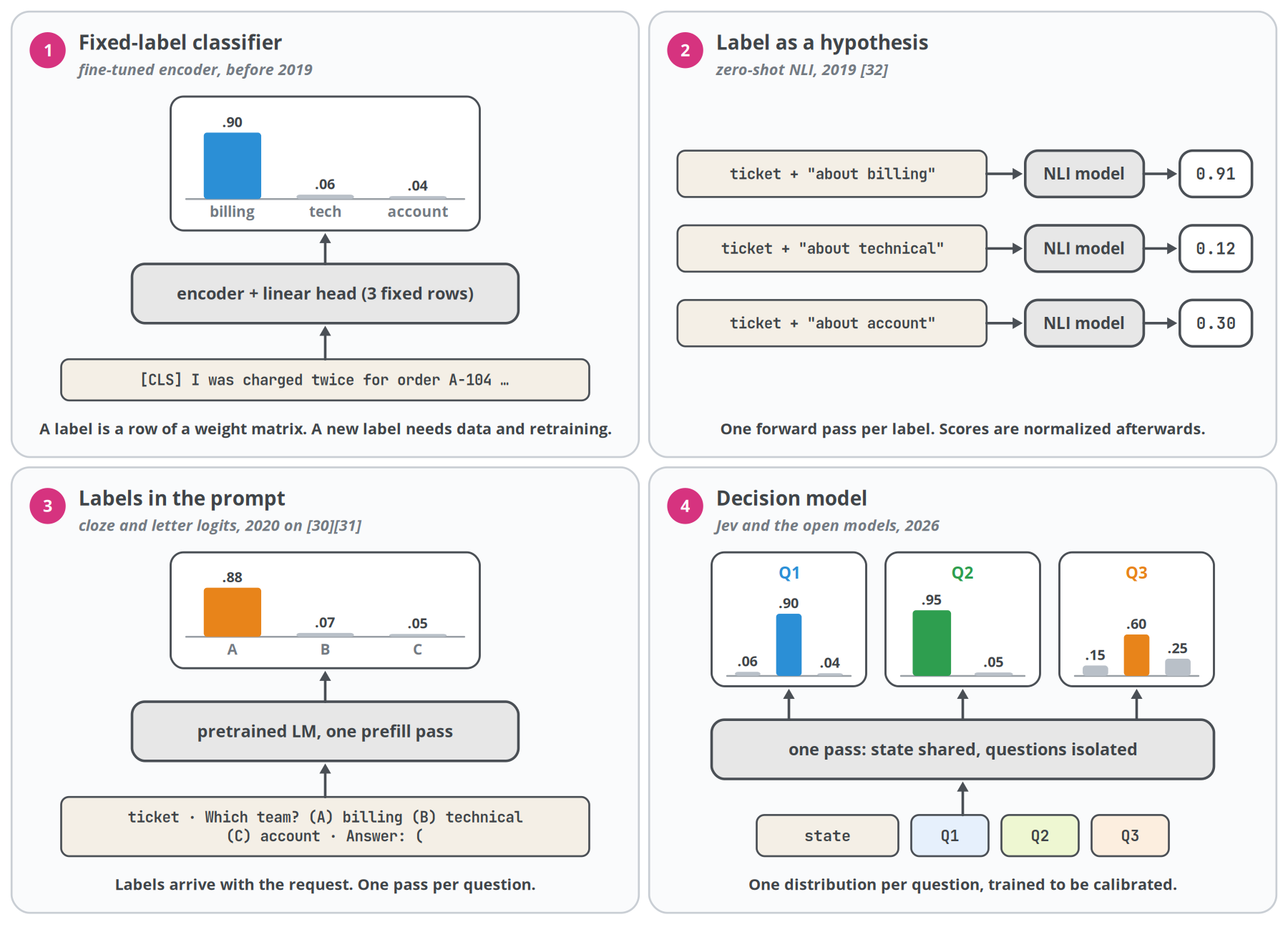
Step 1: a classifier with fixed labels
The standard recipe for ticket routing is an encoder that produces a vector for the whole input, followed by a linear layer with one row per label and a softmax. For our ticket, the layer has three rows: billing, technical and account.
Each label exists only as a learned row of the weight matrix. The model never reads the word "billing". This has several consequences. Adding a fourth label, for example fraud, needs labelled examples and a new training run. A second question about the same ticket, such as whether the customer asks for a refund, needs a second head or a second model. And the probabilities are whatever cross-entropy training produced, which for modern networks tends to mean overconfidence [33].
Step 2: put the label into the input
In 2019 Yin, Hay and Roth recast classification as natural language inference [32]. The ticket is the premise, and each label becomes a hypothesis written in words: "This text is about billing." A model trained on entailment scores how strongly the premise supports each hypothesis, and the label with the highest score wins.
Labels are now text, so any label works at inference time without retraining. There are, however, downsides. Ten candidate labels mean ten passes over the same ticket, and because each pass is independent, the model never compares the labels with each other. The scores become a distribution only after you normalize them.
Step 3: put all the labels into one prompt
A language model can read every option at once. Write the options into the prompt with letters, end the prompt where the answer letter would come next, and read the model's next-token probabilities for the letters. PET did this in 2020 with masked language models and cloze prompts [30]. With a decoder, the prompt simply ends in Answer: (.
One pass now answers one question, and the model sees all options side by side. The following year, Zhao and colleagues found a catch: the probabilities of label tokens are biased toward some labels regardless of the input, for example labels that appeared often or recently in the prompt, and they need correction before they mean anything [31]. In 2026, SemIf uses exactly this method on Qwen3.5-4B, with no training at all [11].
Step 4: many questions, one state, calibrated answers
A decision model in the sense of this book adds four things to step 3. It answers many questions about the same state in one call, and reads the state only once. It keeps the questions independent of each other. It is trained so that its probabilities are calibrated, meaning that answers given with probability 0.8 are right about 80% of the time. And it exposes a typed interface, so that the application receives only values from the declared answer set.
Jev's mechanisms are not new
None of the individual mechanisms is new; the oldest date from 2019. A review by the blogger zephel01 of the first seven Jev reproductions concluded that they copied a "computational form" already described in papers from 2020 and 2021 [25]. Other ancestors show up in later chapters. MiniCheck read a single yes/no token to check facts in 2024, and Bespoke Labs built its Nimble model on that work [39][13]. GLiNER encoded labels as tokens next to the text in 2023 and led to GLiNER2.5-Decide [29][16]. FIRST ranked passages from the logits of a single token [37].
What changed in September 2026 was the combination: one model that accepts arbitrary questions across many domains, training aimed at calibrated probabilities, serving that answers hundreds of questions against one shared state, and a small public API that dozens of projects copied within days. Every model in this book is built to satisfy that API [2][3]. A request carries a state, the evidence to judge, such as our ticket, and one or more typed questions. A Choice picks one option from a set, a Score places the state on an ordered scale whose levels the caller describes, and a Noul is a yes/no question answered with the probability of yes. The model returns a probability for every allowed answer and generates no text.
Chapter 4
How to make a simple decision model
Prefill and decoding
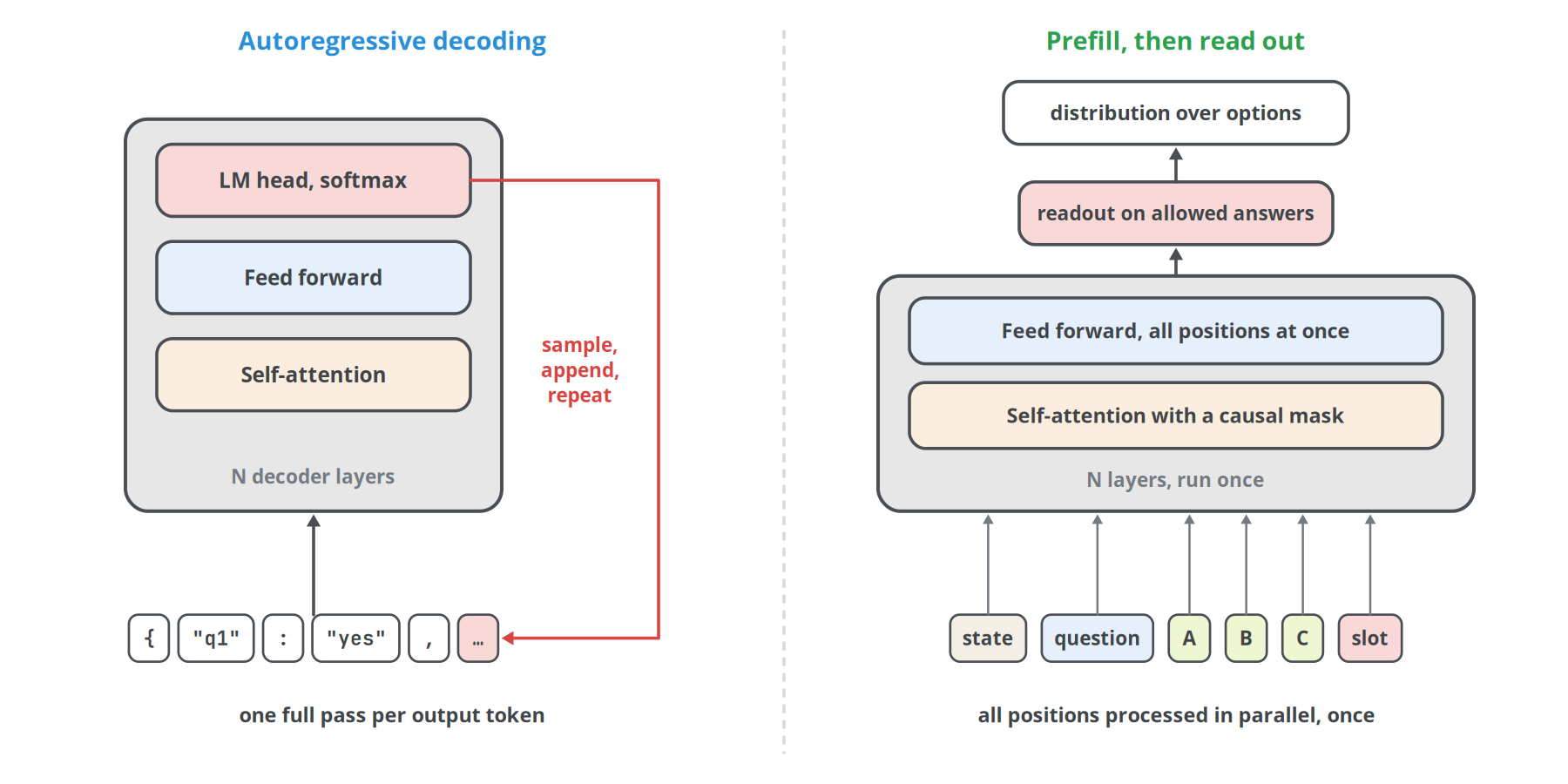
If you work with LLMs, you may have noticed that speed is usually reported as two values: prefill, also called prompt processing, and generation, also called decoding. Per token, prompt processing is usually much faster. Why?
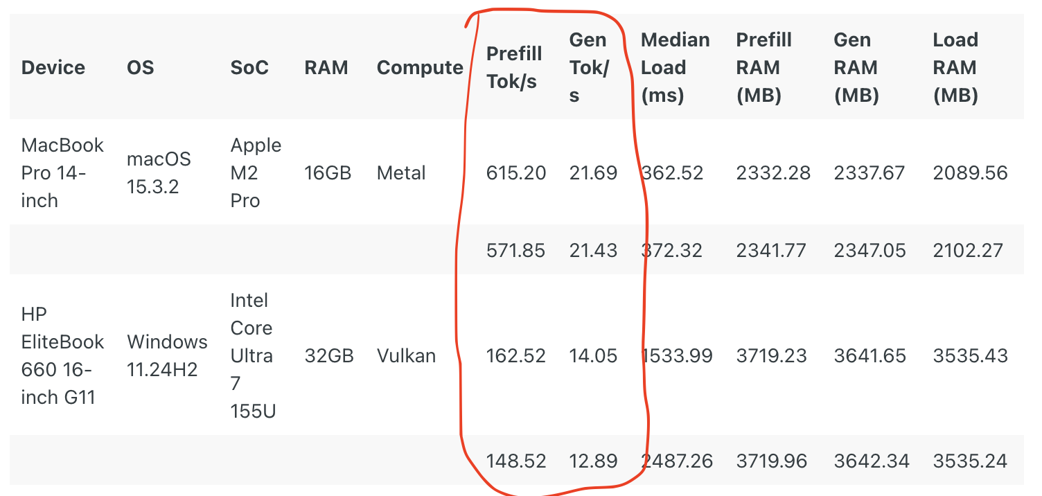
In every LLM, during prefill every input token is already known, so each layer processes all positions at once while a causal mask controls which positions may read which. Hume puts it this way: causal attention describes which positions can use which information, and says nothing about the order in which positions are computed [9]. Decoding is different. Token t + 1 cannot be computed until token t has been chosen, so the network runs once per output token.
A decision model is fast because it processes the whole input at once and generates nothing. It stops after prefill, takes the final hidden vector at one or more chosen positions and turns it directly into scores for the allowed answers.
Getting decision probabilities from the model
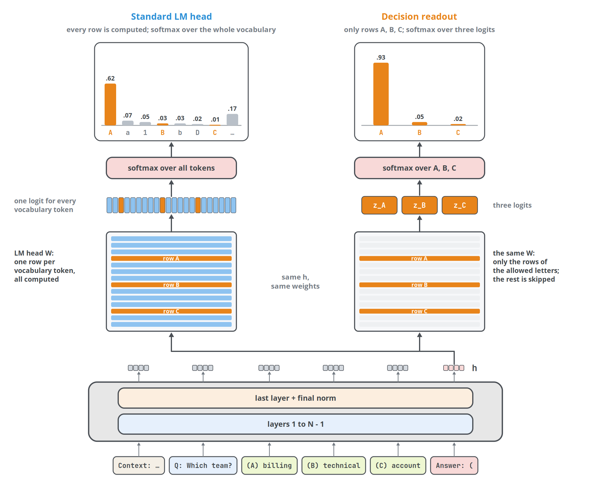
The cheapest readout reuses the network's own output layer. The prompt lists the options with letters and ends where the answer letter would come next. The final hidden vector h at that position normally goes through the LM head, a matrix with one row per vocabulary token, to produce next-token logits. A decision model computes only the rows for the allowed letters. If wk is the row for letter k and T is a temperature,
pk = exp(wk · h / T) / Σj exp(wj · h / T)
Qwen3.5 has a vocabulary of about 248,000 tokens [52], and this computation uses three of those rows. SemIf applies this readout to a frozen model and trains nothing [11]. JevK5 uses the same readout and prompt, adds a low-rank adapter, known as LoRA, to the attention layers, and fits a temperature [12][42]. Bespoke Nimble gives each allowed answer a code that the tokenizer treats as a single token and reads the logits of those codes [13].
Why is this simple approach limited?
The answer-letter readout is cheap and needs no new parameters, but it has several weaknesses, and each design in Chapter 5 removes one of them.
First of all, language models prefer certain answer letters and positions regardless of content, an effect Zheng and colleagues documented on multiple-choice benchmarks [38]. Reordering the options of our team question can change its probabilities.
A common fix at inference time is to ask each question twice, once with the options in reverse order, map the second distribution back to the original order and average the two. A list averaged with its reversal still leaves the middle options in the middle, so this reduces order sensitivity without removing it. Chapter 6 shows how both orders can share one forward pass, and Chapter 14 measures the effect [52].
The probabilities are conditional on the options offered. If the ticket belongs to a team that is not on the list, the model still has to spread its probability over billing, technical and account. SemIf's documentation warns that such a softmax is not a calibrated confidence until it is measured and corrected [11].
The row for the letter "A" was trained to predict the next token of text. Reading it as a classifier weight relies on the base model's habits, which is why every project that uses this readout either fine-tunes the model or at least fits a temperature.
Finally, the number of options is limited by how many distinct single-token codes you can find, and every extra option makes the prompt longer.
Several questions in one pass
Decider extends the readout to many questions. The prompt contains the context once, followed by each question with its lettered options and its own answer slot written as Answer 1: (, Answer 2: ( and so on. One prefill produces a hidden vector at every slot, and each slot is read through the rows for its own letters [14].
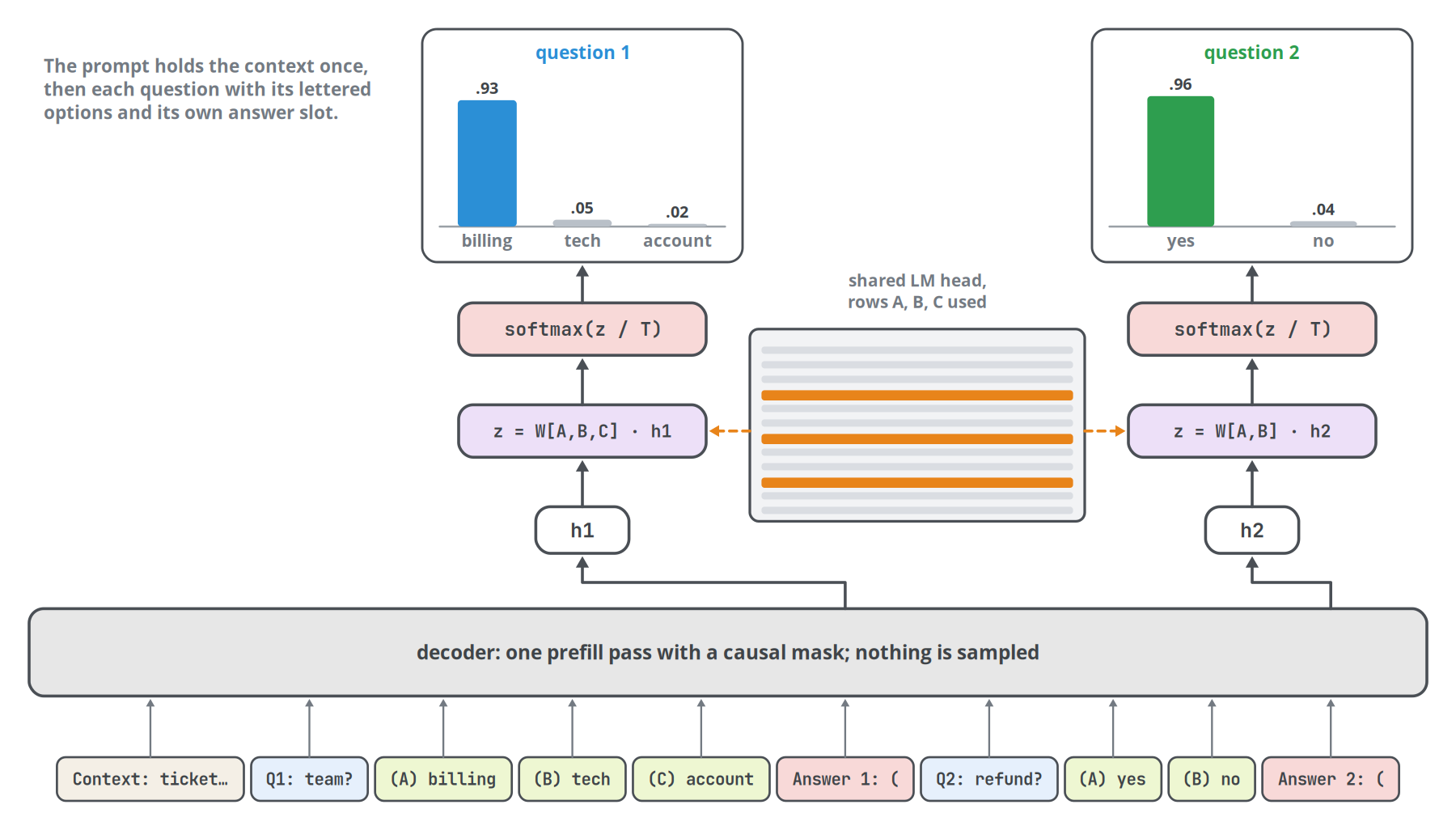
This layout has a side effect worth noticing. In a plain causal pass, the slot for question 2 comes after question 1 and can attend to its text. The answers stay separate, since no letter is ever generated, but the second question's reading can be influenced by the first question's wording. Chapter 6 shows the attention mask that removes this influence.
Reading the answer before the last layer
The readout uses the hidden vector after the last layer. The same LM head, after the model's final normalization, can also be applied to the hidden vector after any earlier layer. This probe, known as the logit lens, shows at which depth the answer becomes readable through the unchanged head, with nothing new trained [55]. A tuned lens trains a small map for each layer and can read the answer earlier, because it does not require the intermediate representation to already match what the final head expects [56].
If the answer is readable early, the forward pass can stop early. An early-exit model adds a light head after selected layers and stops when that head's confidence passes a threshold chosen on held-out data, a technique studied for generative models under names such as confident adaptive language modelling [57]. Decision models face two practical limits. A batch can stop only when every request in it has stopped, and a captured CUDA graph (Chapter 6) has to be split at every exit. The gain is also bounded by where the decision forms: if it becomes readable only in the last tenth of the network, no exit saves more than about a tenth of the work. Chapter 14 reports exactly that case.
Chapter 5
More advanced ways to read answers
Each design in this chapter starts from one weakness of the letter readout and removes it, at a cost that the design's authors document.
The five designs appear in the order of how far they move from an ordinary decoder. All five use the running example: the team question with three options, and the refund question with two.
A pointer head: score the options themselves
Kev, built by Jared Palmer, drops the letters [10]. Every option ends with a reserved end-of-option token, and each question ends with a reserved <decide> token. After prefill, the model takes the hidden vector at each option's end token, ok, and the hidden vector at <decide>, d. Two small linear maps project them, and the score of option k is the dot product of the two projections. A softmax over the scores of one question gives that question's distribution.
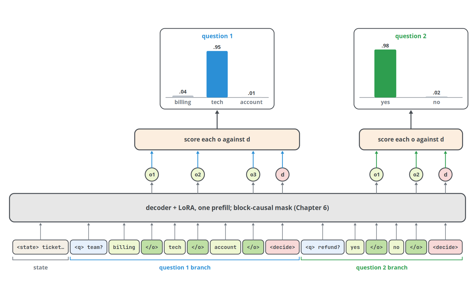
Two properties follow from where the tokens sit. The option's own representation is scored, so no letter carries a prior preference. And because <decide> comes after all options, d has read the complete list when the scores are computed, which is what lets an option such as "none of the above" work. The number of options is whatever the request contains.
The head is new and must be trained. Kev trains it from scratch together with a rank-16 LoRA on the backbone, using cross-entropy on the option distribution [10]. Order effects remain smaller but present: across four option orders, Kev's answers changed 7.4% of the time.
Option markers in an encoder: a small model that compares options
Laya, from Convai Innovations, uses a bidirectional encoder in place of a decoder [15]. The input is the state, the question, and each option preceded by a [MASK] token. ModernBERT-large encodes everything in one pass, and every token can attend to every other, so options, question and state all see each other [44]. The hidden vectors at the mask positions go through a decision head of two transformer layers, and an option scorer turns each into one logit. A separate head reads the [CLS] vector and estimates whether the system should act at all.
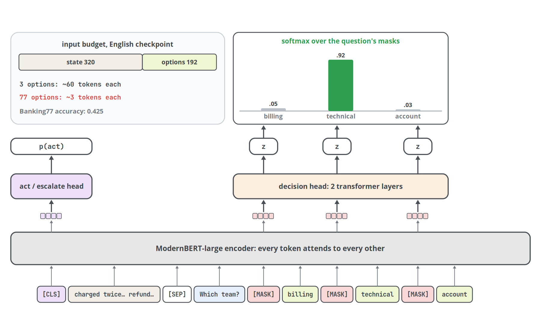
The model has 421 million parameters and answers a call in 33 to 40 ms on a T4 GPU. Its fixed input size is the main cost. The English checkpoint reserves 192 of its 512 tokens for options, so 77 options receive about three tokens each; on the Banking77 intent benchmark, accuracy falls to 0.425 [15]. The model card also reports that the base checkpoints score close to chance on its typed-decisions benchmark until they are fine-tuned on the domain, and that the act head carries no usable signal yet.
Label tokens and a joint decoder: answers that must agree
Some questions constrain each other. If a guardrail finds a prompt injection in our ticket, it should not also call the ticket safe. Scored independently, those two questions can contradict each other.
GLiNER2.5-Decide from Fastino addresses this case [16]. It descends from GLiNER, which writes each task and each candidate label as special tokens next to the text: [P] marks a task and [L] marks a label [28][29]. A DeBERTa-v3-large encoder reads the schema and the text together, and a small head computes a compatibility score for every label [45]. On top of the scores sits a decoder. The schema can declare rules such as implications, exclusions and limits on how many labels may be chosen, and the decoder searches for the highest-scoring combination of answers that satisfies them.
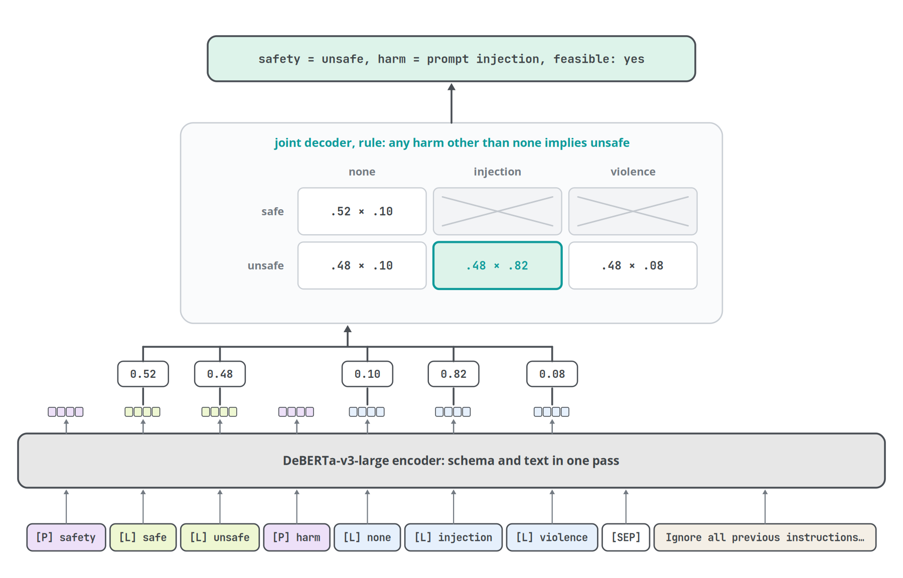
Fastino reports a median latency of 38 ms on a V100 GPU and 167 ms on a 48-core CPU. The same pass can also return character offsets for extracted entities [16]. An independent evaluation by the GitHub user turlockmike found that the shipped probabilities were overconfident, and suggested a reason: the open-source trainer uses a separate binary loss per label, while single-label inference applies a softmax across labels [24].
A dual encoder: many candidates, reused across steps
An agent playing a game or calling tools faces the same set of actions at every step while the state changes. Reading all candidates again at every step wastes work.
CLM-8B, from Stanford's Scaling Intelligence Lab and NVIDIA Research, encodes states and actions separately [18]. A frozen Qwen3-8B turns the state into one vector and each candidate action into another. Two projection heads of about 20 million parameters each map them into a shared space, and the score of an action is a scaled dot product with the state vector. A softmax over the candidates gives the distribution. Action vectors do not depend on the state, so they can be computed once and cached.
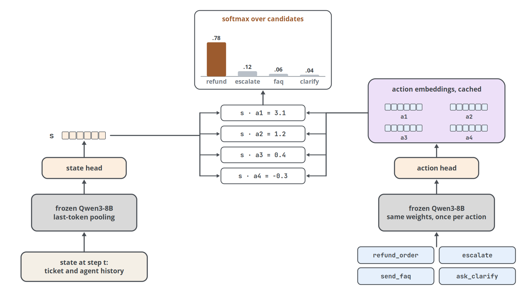
The cost is that state and action meet only in the final dot product. Inside the network they never attend to each other, so fine-grained interactions between a particular action and a particular detail of the state are harder to capture. The team's reported comparison with Jev shows the trade: 16.5 ms per decision against 149.8 ms on a simple game with equal success, but 26 of 30 Wikipedia navigation tasks completed against Jev's 30 [50].
A diffusion canvas: no training at all
A diffusion language model generates text by starting from masked tokens and refining all of them in parallel over a few steps. DiffusionGemma is such a model, a Gemma 4 mixture-of-experts network with 3.8 billion active parameters, fine-tuned to refine blocks of 256 tokens at once [49].
The open-jev harness by JoshuaSP writes the questions as a JSON template, leaves each answer slot masked, runs one to four denoising steps and reads the most likely allowed token at every slot [19]. Nothing is trained.
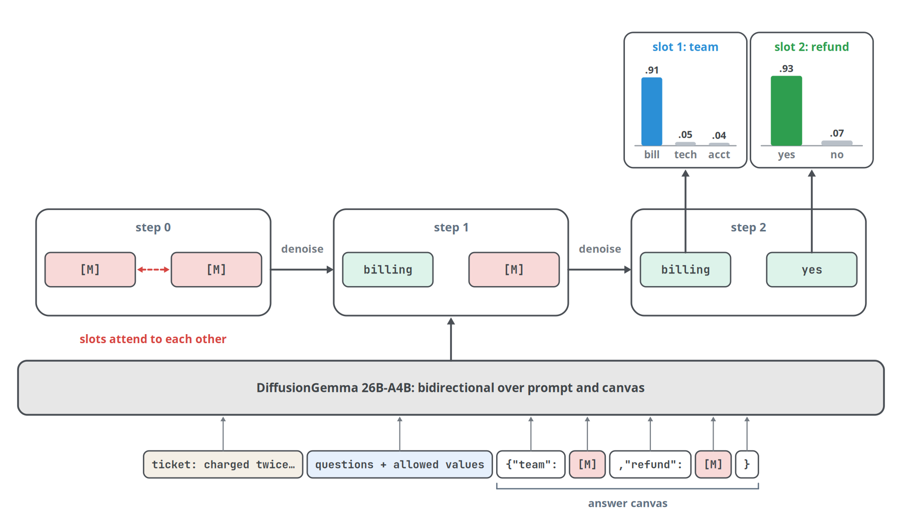
The canvas has the opposite property to Kev's branches: every answer slot attends to every other. Adding a question can change the answers to the other questions. The model is also large, 26 billion parameters in total.
The designs side by side
| Design | Trained parts | Options compared inside the network | Questions kept separate | Options per question | Example size |
|---|---|---|---|---|---|
| Answer letters | none, LoRA, or all weights | yes | only with a mask or separate passes | limited by single-token codes; Nimble allows 255 | 4B to 35B |
| Pointer head | LoRA and a new head | yes, decide token reads the list | yes, block-causal mask | any | 0.5B to 9B |
| Encoder markers | all weights and a head | yes, bidirectional | not documented | limited by the option budget | 322M to 421M |
| Label tokens and joint decoder | all weights | yes, bidirectional | no, joined on purpose by rules | limited by context | 340M to 576M |
| Dual encoder | two projection heads | no, only through the dot product | yes | thousands, cached | 8B frozen |
| Diffusion canvas | none | yes | no, slots share attention | limited by canvas length | 26B |
Every design above still has to read the state. When the state is long and the questions are many, how the state is shared between questions decides most of the cost, which is the topic of Chapter 6.
Chapter 6
Optimization techniques
Sharing the prefix
In a transformer, the stored representations of processed tokens are the keys and values of every attention layer, the KV cache. If the state comes first in the sequence, its KV cache can be computed once and reused by every question that follows.
Hydragen and DeFT showed how to compute attention efficiently when many sequences share a prefix or form a tree [35][36]. SemIf measured the gain on a workload of 37 states of about 8,000 characters, each with the same 21 questions [11]. Scoring every decision from scratch ran at 2.33 decisions per second. Prefilling the state once and scoring the questions one after another reached 10.75. Scoring all questions as parallel branches on the shared prefix reached 20.03.
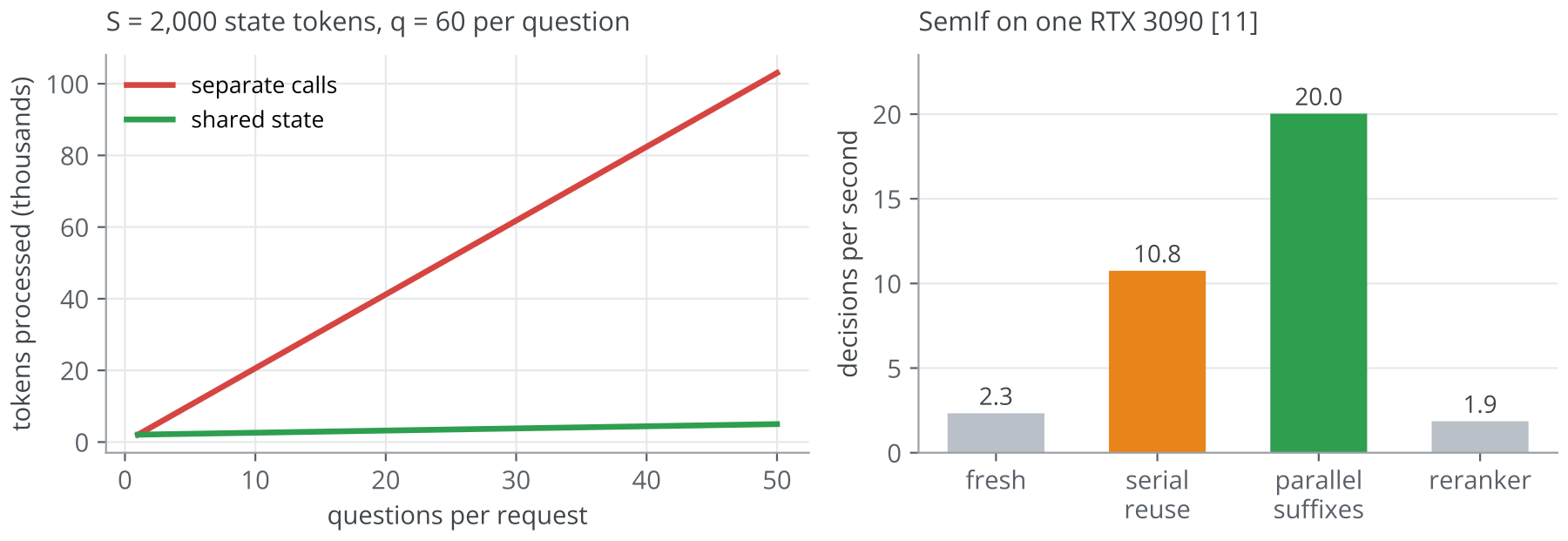
SemIf also reports a side effect. In 16-bit floating point, the faster paths changed the winning answer in 5 or 6 of 777 decisions compared with scoring from scratch. Different kernels round differently, and a close call can flip.
The block-causal mask
Kev implements sharing inside a single packed sequence [10]. The state comes first, followed by each question as its own branch: a question token, the instructions, the options with their end tokens, and a <decide> token. A standard causal mask would let question 2 read question 1. Kev's mask adds one condition. Position i may attend to position j only if j comes before i and j is either part of the state or part of the same question as i.
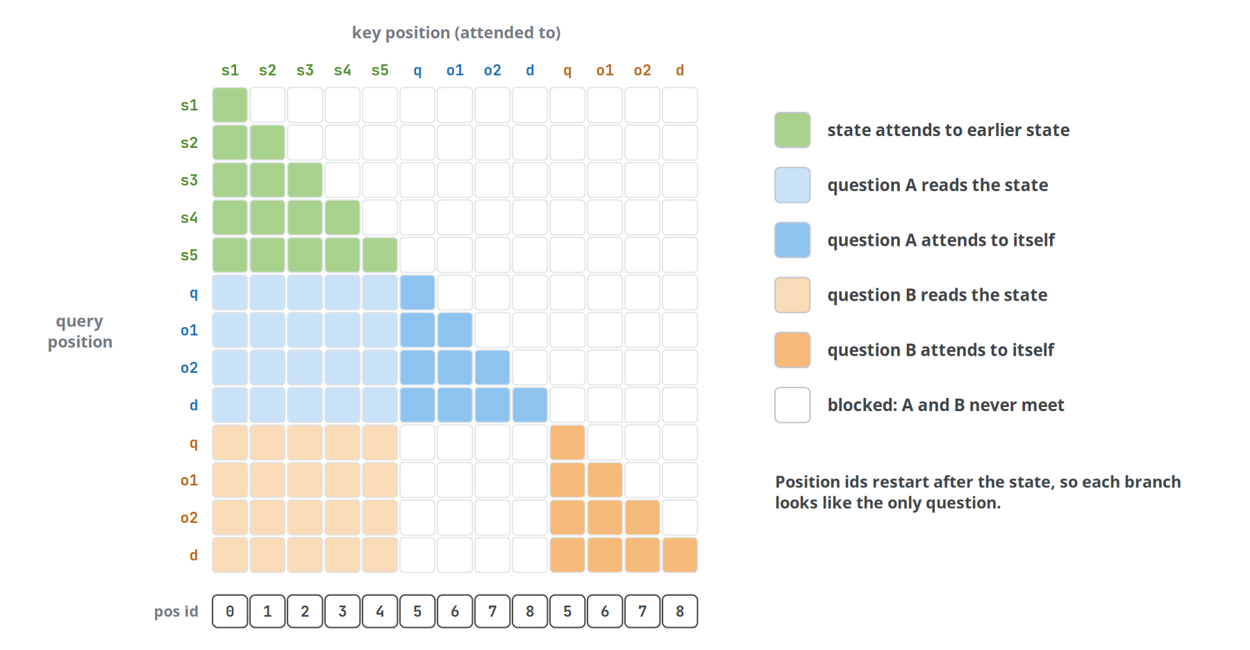
Position ids also restart after the state, so every branch looks to the model as if it were the only question in the sequence. The order of questions in the request no longer matters.
The same mask serves a second purpose. To average over two option orders (Chapter 4), a model can pack the shared prefix once, followed by the options in the original order and the options in the reversed order. The positions of both option blocks continue from the end of the prefix, and the mask keeps the two blocks apart. One forward pass then yields both readouts at nearly the cost of one; basal-1.0 measured 12.5 ms for both orders against 11.6 ms for a single order on an H100 [52].
Kev's authors tested the isolation directly. They placed a secret code in one question and asked another question to report it. The probe gave the code a probability of 0.03, the same as when the question containing the code was removed. With the code moved into the state, the probability rose to 0.99. Packing six questions into one sequence gave probabilities within 3.7 × 10⁻⁶ of answering them one at a time, and ran twice as fast [10]. The branch delimiters are reserved tokens, so text inside the state cannot imitate them and create a fake question or option.
Why isolation matters
Isolation gives the API its meaning. Whether our customer sounds angry should not change which team receives the ticket. With isolated branches, you can add a monitoring question to a production request without changing any production answer. Isolation also has a security side: the text of one question cannot manipulate another question's answer [10].
Not every system provides it. The diffusion canvas from Chapter 5 lets answer slots attend to each other, and the OpenJev server built on it deliberately re-reads all questions when one answer is uncertain [19]. Neither choice is wrong, but you need to know which one you are running before assuming that answers stay stable when you edit other parts of a request.1
Tokens are the unit of cost
Every state token passes through every layer, so the tokenizer sets the price of a decision. Tokenizers trained mostly on English split other languages into more pieces. On identical Polish decision prompts, the multilingual tokenizers of several popular open models needed 17% to 51% more tokens than a 32,000-token tokenizer built for Polish [52]. How much that costs depends on how the model is served. At batch size 1, a 4.5B model's latency stayed flat up to about 1,000 tokens, because fixed costs per layer dominate. At a server batch of 32, throughput fell almost in proportion to prompt length, so the longer encodings meant 15% to 34% fewer decisions per second on the same GPU [52].
Making one forward pass fast
A decision costs one prefill, and at batch size 1 the arithmetic is small: about 4 TFLOP for a 4.5B model on a 400-token prompt, a few milliseconds on an H100. A plain PyTorch forward pass in bf16 nevertheless took 32 ms in the basal-1.0 measurements, because the GPU spent most of that time waiting for thousands of small kernels to be launched one by one [52]. The techniques that remove this overhead are generic and apply to every decision model in this book.
A CUDA graph records the kernels of a whole forward pass once, for a fixed input shape, and replays them with a single launch. Inputs are padded to a small set of shapes, for example batch sizes from 1 to 32 and lengths in steps up to a few thousand tokens. With causal attention, padding placed after the last real token cannot influence it, so the readout takes the hidden state at the last real position. Compilation fuses small operations such as normalizations, rotary embeddings and activations into fewer kernels before the graph is captured. Batching by token budget sorts waiting requests by length and cuts them into batches whose padded size stays under a fixed number of tokens; padding a batch of 32 to its longest prompt had wasted up to two thirds of the compute [52].
Lower precision helps only where arithmetic or memory traffic is the bottleneck. In FP8 each weight and activation takes one byte [60], and in 4-bit formats such as NVFP4 half a byte. A machine can be limited by kernel launches, by compute or by memory bandwidth, and the best precision differs between them. On a data-centre GPU where a 4.5B model is launch-bound, quantization only adds work. On a desktop machine that must read all 9 GB of bf16 weights for every forward pass through about 273 GB/s of memory bandwidth, FP8 halved the latency. Quantization also changes some decisions, about 3% for FP8 and 10% for 4-bit in the basal measurements, so a calibration fitted in bf16 has to be checked again [52].
Same request, same answer
A decision model should return the same probabilities for a request whether it runs alone or inside a batch. In 16-bit arithmetic this is not guaranteed: the order of floating-point operations can depend on the batch shape, and rounding differences can flip a close call, as the SemIf measurements earlier in this chapter showed. Mixture-of-experts models are especially exposed. In such a model a small router network picks, for every token, which few of many expert feed-forward blocks process it. A tiny rounding difference can change that choice, and a different set of experts gives a different answer. One mixture-of-experts model evaluated for basal-1.0 changed a single prompt's probabilities by up to 0.37 with the composition of the batch in bf16, and not at all in fp32 [52]. The practical safeguard is a parity check: score each prompt alone and inside a batch, and refuse the configuration if the probabilities differ by more than a small tolerance, 0.02 in basal-1.0.
Jev behaves as if it were built this way. Chapter 10 shows the experiments behind that statement. Before that, Chapters 7 to 9 cover the other half of a decision model: whether its probabilities can be trusted, and how training makes them trustworthy.
Chapter 7
Calibration
A weather forecaster says "70% chance of rain" on a hundred different days. If it rains on about seventy of them, the forecaster is calibrated, even though every single forecast was either right or wrong.
The same test applies to a decision model. Take every answer it gave with probability around 0.7, and count how often those answers were correct. If the count is near 70%, the probabilities mean what they say, and an application can act on them. A router that is right 90% of the time without being able to say which 10% is wrong forces a team to review every ticket.
What calibration means
A model is calibrated when, for every probability level p, the answers given with probability p are correct a fraction p of the time. Calibration describes a group of predictions. It says nothing definite about one answer, and TypeSafe's documentation makes the same point [2]. A model can also be calibrated and useless: a router that always answers "billing" with probability 0.6 is calibrated if 60% of tickets go to billing.
Calibration and accuracy are separate properties. Accuracy counts how often the top answer is right. Calibration asks whether the stated probabilities match those frequencies. Temperature, introduced in Chapter 4, changes calibration without changing accuracy at all.
Measuring it
The usual picture is a reliability diagram. Sort predictions into bins by the probability of the chosen answer, typically ten bins of width 0.1, and plot each bin's average probability against its observed accuracy. A calibrated model lies on the diagonal.
The expected calibration error, ECE, compresses the diagram into one number: the average gap between probability and accuracy across bins, weighted by the share of predictions in each bin [33]. The Brier score is the squared distance between the predicted distribution and the one-hot outcome, averaged over examples. It rewards accuracy and calibration together, and lower is better.
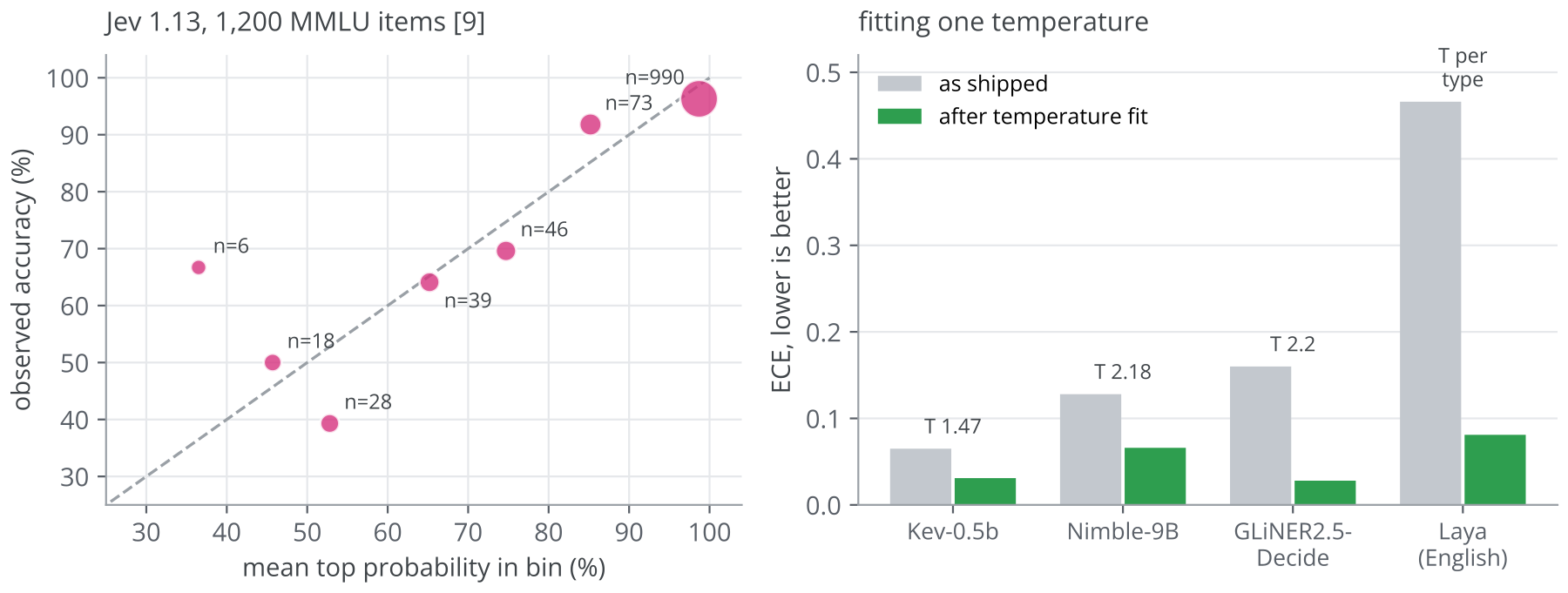
ECE has two blind spots. Overconfidence in one bin and underconfidence in another partly cancel. And if almost all predictions fall in the top bin, ECE mostly measures that bin. Hume's reliability data for Jev shows both effects: an ECE of 0.031 on 1,200 MMLU questions, with 990 of them in the 0.9 to 1.0 bin and the lower bins based on a handful of items each [9].
Temperature scaling
The standard fix is to divide all logits by a single constant T before the softmax, and to choose T by minimizing the log loss on held-out data [33]. A value above 1 flattens distributions; a value below 1 sharpens them. The winning answer never changes, so accuracy stays the same.
Almost every open decision model ships overconfident at T = 1, and the fitted values are large. Bespoke Nimble uses 2.179, GLiNER2.5-Decide needed 2.2 in turlockmike's evaluation, JevK5 uses 1.532 and the original Kev used 1.47 [10][12][13][24]. Decider fits one temperature per question type [14], and Laya fits one per question type and number of options, which brings its English checkpoint's ECE from 0.466 to 0.081 [15].
Why temperature fitting goes wrong
A team routes tickets with a Noul threshold of 0.8 on "refund requested", tuned in the first week. Then someone fits a temperature of 2.2, and the share of automatically approved refunds drops by half overnight. Nothing was wrong with the fit. Temperature does not change which Choice option wins, but it changes every Noul probability and every Score expectation, so every threshold tuned before the fit has to be tuned again. Bespoke Labs' release notes warn about exactly this [13].
A single temperature can also help the average and hurt a subgroup. Nimble's fit improved average calibration, while the ECE of its Score questions rose from 0.105 to 0.177 [13].
The third failure is distribution shift. Laya's English checkpoint scored 0.000 accuracy on Khmer text while reporting 0.952 confidence [15]. No threshold on confidence can catch that. Kev's model card states the general rule: calibration measured on the training datasets says nothing about a new workflow, which needs its own labelled outcomes [10].
Risk and coverage
For a product decision, the most useful curve is neither ECE nor the reliability diagram. It is accuracy as a function of coverage, the share of cases the model decides alone. turlockmike measured this for GLiNER2.5-Decide after temperature scaling: the 50% most confident answers were 84.8% accurate, and the 30% most confident were 91.0% accurate [24]. zephel01 reports similar numbers from his own tests of Jev: a threshold of 0.95 gave 96.8% accuracy on the automated cases, and only 25.8% of cases were automated [25]. Those two numbers, accuracy on what you automate and how much you automate, are the ones a team negotiates over.
How the threshold is chosen decides whether such numbers can be trusted. A curve read off the test set afterwards shows what was possible, not what a deployed system would have achieved. The sound protocol picks the threshold on a separate calibration split, freezes it, and only then measures on the test split both the share of cases accepted and the error actually observed among them. This is selective classification in the sense of Geifman and El-Yaniv [61]. Chapter 14 shows how far a frozen operating point can land from the curve read afterwards [52].
In the same author's test of 480 four-way questions, Jev's middle confidence bands were poorly calibrated: answers in the 0.7 to 0.8 band were correct only 50% of the time [25]. Comparisons between Jev and open models depend heavily on the benchmark. On JevBench's calibration axis, as quoted by zephel01, Jev scored 82.7 against 72.6 for SemIf and 42.0 for Kev-4B [25]. On the Decision Index 0.2 sample, Jev's ECE was 0.074 while AutoJev-27B reached 0.018 and JevK5 0.027 [22]. The benchmarks use different items and definitions, so the only safe conclusion is to measure calibration on your own data.
Chapter 8
Training for decisions
Temperature scaling repairs calibration after the fact. Training decides how much repair is needed, and whether the model knows anything worth calibrating.
The loss: cross-entropy over the allowed options
Most open decision models are trained with cross-entropy computed only over the options that the question offers:
L = − log pθ(y | state, question, options)
where y is the correct option.
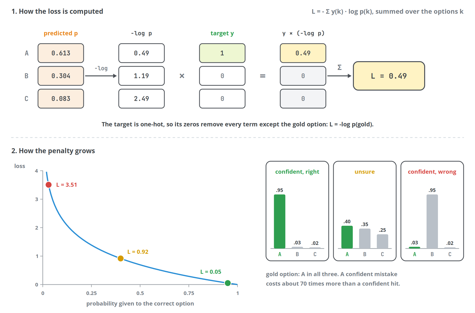
Kev, JevK5, Nimble and Decider all use this loss [10][12][13][14]. It has a property that matters for calibration: it is a strictly proper scoring rule. A scoring rule assigns a reward to a reported distribution once the outcome is known. It is proper if the expected reward is highest when the reported distribution equals the true one, and strictly proper if no other report does equally well [34].
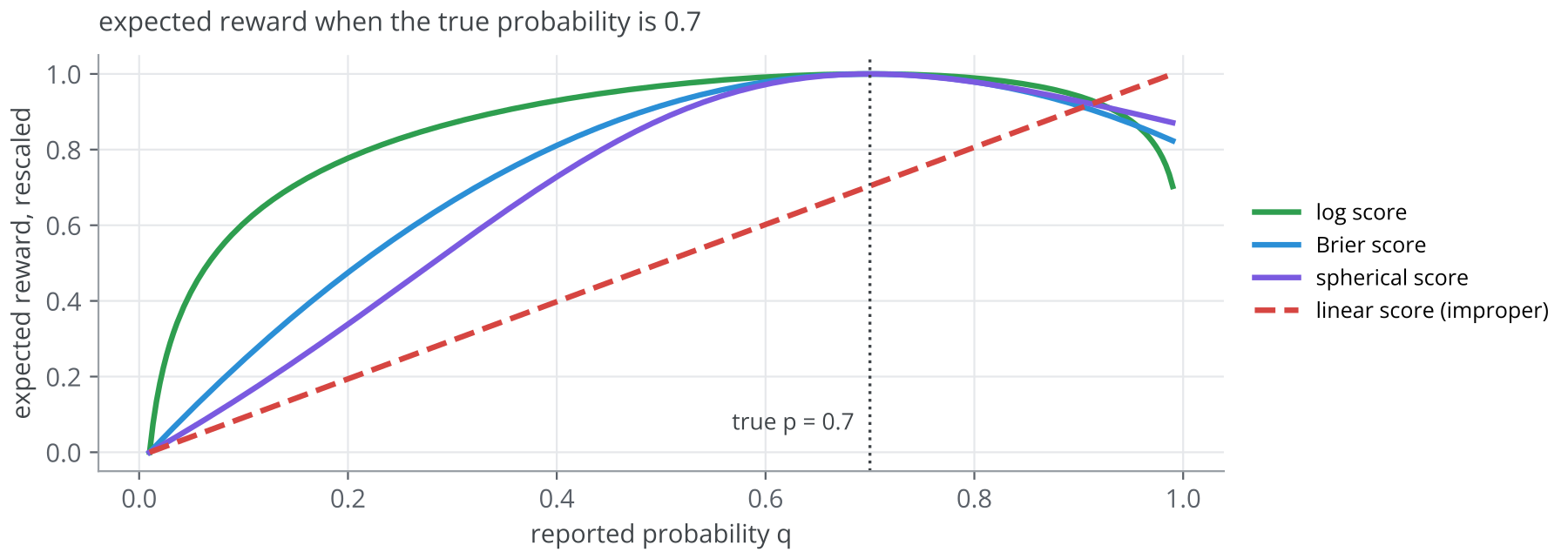
| Scoring rule | Reward for outcome y | Where it appears |
|---|---|---|
| Log score | log q(y) | cross-entropy training in most projects; part of Laya's reward |
| Brier score | minus the squared distance between q and the one-hot outcome | calibration metric in model cards and in JevBench |
| Spherical score | q(y) divided by the length of the vector q | part of Laya's reward |
| Ranked probability score | squared error of cumulative probabilities over ordered levels | Laya's reward for Score questions |
When the reference answer is itself a distribution, the same loss becomes a cross-entropy against that distribution. JevK5 includes a small pilot of such items [12]. Decider's second training stage uses the idea to prevent forgetting: rows replayed from the first stage are trained toward the first-stage model's own distribution with a KL term, and new rows are trained on their labels [14].
Training data also has to teach the invariances an API user expects. Kotoba Labs' open-jev-deberta shuffles options, paraphrases instructions, drops distractor options, relabels Score levels and negates Noul questions while flipping the label [27]. Kev can add a KL term between predictions under two option orders, and an ordinal term for Score questions [10]. Decider trains on two prompt layouts, keeps at most ten options per example with the correct one always included, and adds 10% of rows where the correct answer is to abstain [14].
Training recipes
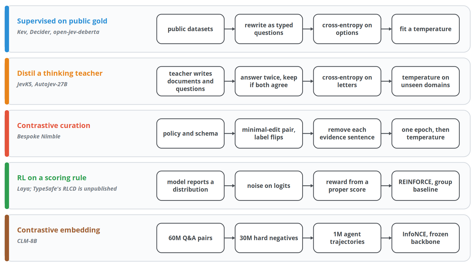
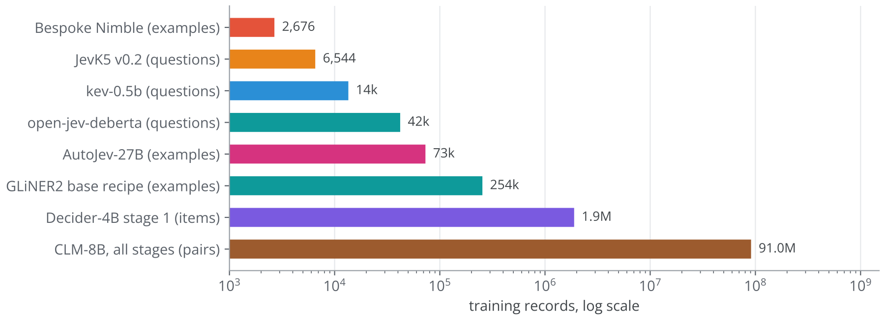
The projects differ mainly in where their labels come from. The figure shows five recipes, and the sections that follow describe four of them in detail; the first, supervised training on public labelled datasets, is the familiar case.
Distilling a model that thinks
A reasoning model that thinks for thousands of tokens answers hard decisions well and slowly. JevK5 tries to move part of that ability into a single pass [12]. Its teacher, Qwen3.6-27B with thinking enabled, writes realistic documents with hard typed questions across 17 business domains: policies with exceptions, traps in dates and numbers, lookups that need several steps, injected instructions and misleading notes. The teacher then answers every question twice, independently. A question stays only if both answers match the intended one, and option keys are rebuilt from the option text so that no key hints at the answer.
The 3,272 surviving questions are mixed with an equal number of human-labelled items from MMLU-Pro, WANLI, MultiNLI, BoolQ, Banking77, ARC and CommonsenseQA. Training is two epochs of cross-entropy on the letter logits. The temperature is fitted on teacher questions from three domains that training never saw: residential leases, public-sector permits and manufacturing quality control. The team also tried one temperature per question type and averaging over two option orders, measured both on held-out data, and rejected both [12].
Distilling a distribution
A teacher can contribute more than its answers. Its whole probability distribution over the options carries information about how close the alternatives were [54]. The student is then trained on a mix of the usual cross-entropy with the gold label and a KL term toward the teacher's distribution:
L = (1 − α) · CE(y, pS) + α · KL(pT || pS)
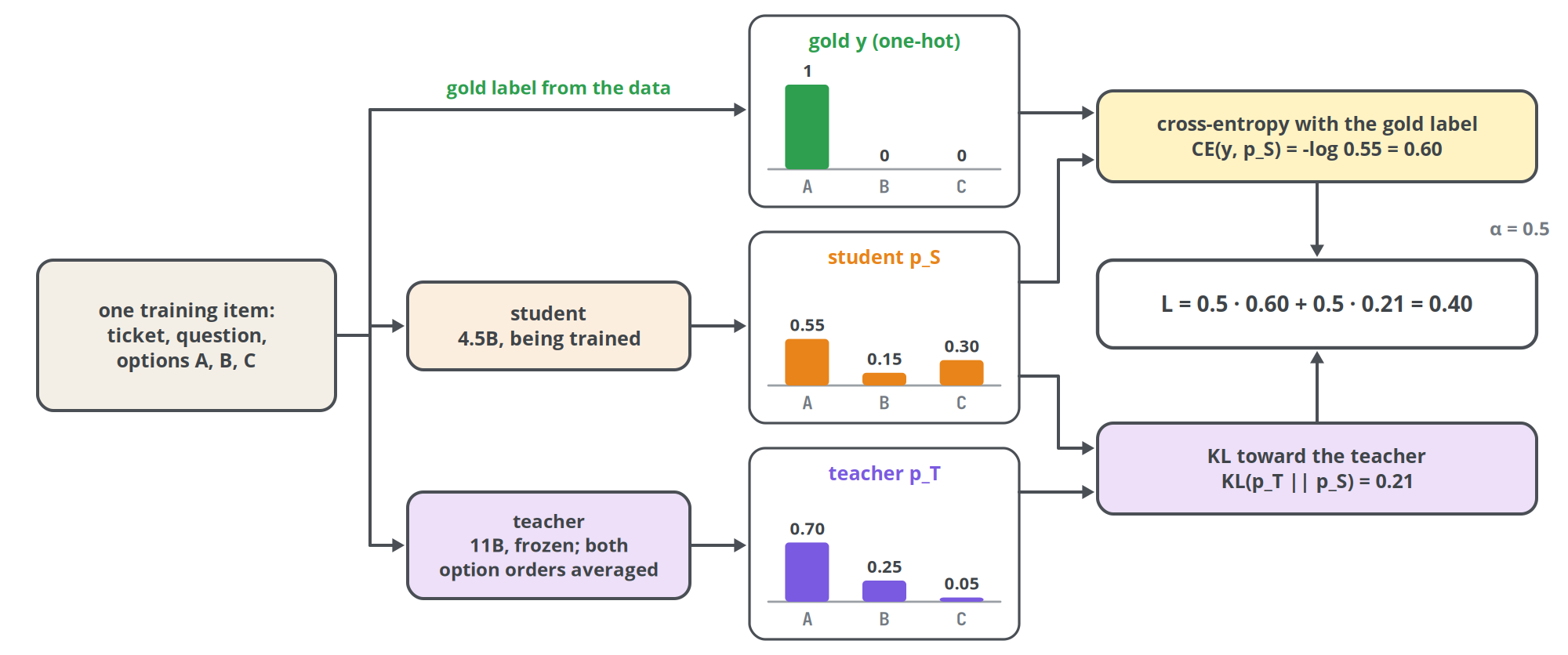
basal-1.0 used α = 0.5, with the teacher's distribution averaged over both option orders, and found that the result depends on the teacher's strengths. Distillation from an 11B teacher improved a date-arithmetic primitive by about 10 points and lowered English accuracy, on which the teacher had not been trained. The rule adopted was to distil only from a teacher that is strong in the domain, and only on items where its top answer is correct. The same loss, with the frozen 4.5B model as the teacher, produced the 1.5B variant [52].
Contrastive curation
Bespoke Labs had no teacher probabilities and did not want to copy Jev, so they built data that forces the model to find the evidence that matters [13]. Each training pair consists of two examples that differ in one fact, changed with at most eight words, and the change flips the correct answer.
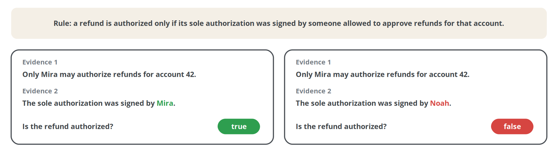
The pipeline checks each pair in four stages. It first confirms that the policy's rules can lead to different answers. It then writes two evidence sentences that are both needed for the answer and edits one of them. Separate model calls verify the facts in each example and check that no wording hints at the answer. Finally, each evidence sentence is removed in turn, and the focus fact must become unknown, which shows that nothing else in the text reveals the label. Code then computes the labels from the checked facts. The method descends from Bespoke-MiniCheck [39]. All labels are synthetic and were checked by models; the team notes that separate calls to one model can repeat the same mistake [13].
A related construction teaches a model to say that a case cannot be decided. An evidence-sufficiency pair asks whether the state contains enough information to decide, once on the full state, where the answer is yes, and once with the deciding fact removed, where it is no. basal-1.0 builds such pairs from its generated cases, and generates rule-based twins in code, so their labels need no model at all [52].
Reinforcement learning on a scoring rule
TypeSafe describes its training method, Reinforcement Learning for Calibrated Decisions or RLCD, only by its goal, which Chapter 10 quotes [5]. Laya published its own method under the same name [15]. The model outputs a distribution over options. For exploration, zero-mean Gaussian noise is added to the logits, which gives a slightly different reported distribution. The reward is a proper scoring rule applied to that report and the known outcome: a mixture of the log score and the spherical score, plus the ranked probability score for Score questions. Updates use REINFORCE [51] with the mean reward of a group of samples as the baseline, the scheme popularized as GRPO [46].
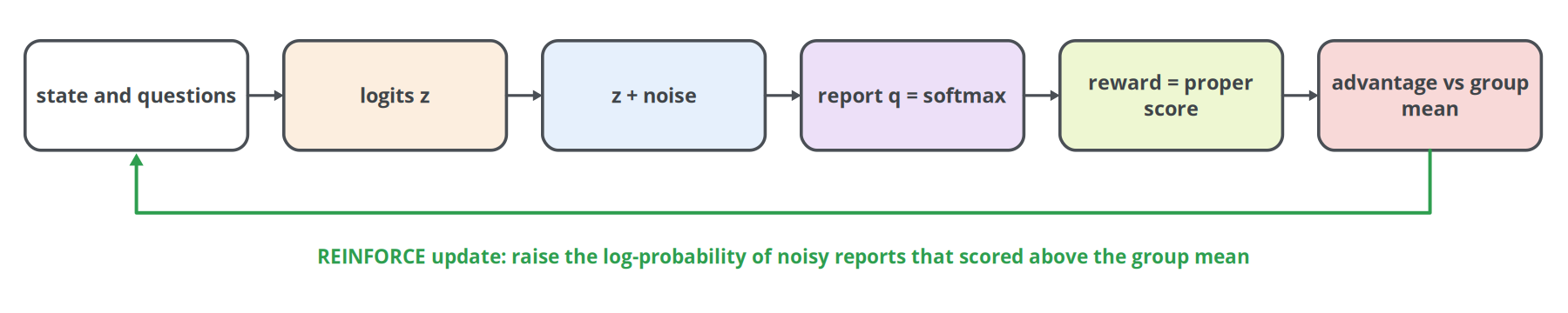
When the labels are ordinary targets available for every example, supervised log loss already optimizes the same expected score as this RL setup, and it does so with less variance than a REINFORCE estimate. RL pays off when the reward is not a label the model can be trained on directly, for example a success signal observed later in a workflow, or a reward over a multi-turn episode. Laya uses the second case for conversations, with TD(λ) over prefixes of the dialogue [15]. Whether TypeSafe's RLCD works like this is not known.
Contrastive embedding
CLM-8B is trained with InfoNCE [41]. For each state in a batch, the embedding of the action actually taken is pulled toward the state embedding, and the other actions in the batch are pushed away; the loss is applied in both directions, from states to actions and from actions to states [18]. The backbone stays frozen and only the two heads learn. Training runs in three stages: 60 million question-answer pairs, then 30 million synthetic hard negatives, then one million agent trajectories. The team reports that the contrastive loss falls as a power law in compute, model size and data [18].
Making a smaller model
An accurate decision model that is too slow can be shrunk in three ways. The first is to distil it into a smaller model of the same family, which shares the tokenizer and was pretrained at its own size. The second is layer pruning, which removes whole blocks of middle layers from the trained model, motivated by work showing that many of the deeper layers of large language models can be removed at modest cost [58]. The third is a looped or recursive transformer, which replaces a stack of layers by one shared block applied several times, sometimes with a small adapter for each pass [59]. basal-1.0 tried all three with one recipe and budget, and only the first worked well; Chapter 14 gives the numbers [52].
The last step
Every recipe ends by fitting a temperature on held-out data, including Laya's, which already trains on a proper scoring rule [15]. A proper loss pushes toward calibration in expectation, and finite data, limited capacity and shift between training and use leave a gap that one scalar closes cheaply [33].
Chapter 9
Data
TypeSafe has not disclosed what Jev was trained on. The open projects publish their data, and together they show what a decision model needs to see.
| Project | Training data |
|---|---|
| kev-0.5b [10] | Banking77, AG News, MNLI, BoolQ, SST-5 and Yelp reviews; 9,000 records with 13,500 questions |
| Kev-4B update [10] | adds TREC, DBpedia-14, Amazon reviews and IMDB, a programmatically labelled hard set, and developer-tooling data from CodeReviewer, CommitPackFT, FlakeFlagger and Aegis |
| JevK5 [12] | 3,272 teacher-written questions in 17 domains and as many human-labelled items from seven public datasets |
| Bespoke Nimble [13] | 2,676 contrastive examples in 10 subject areas: 856 Choice, 888 Noul and 932 Score |
| Decider-4B [14] | about 95 public decision datasets, agent trajectories, Mind2Web, 26 datasets with gold labels in law, tables, logs, medicine and multilingual inference, and 10 programmatic families |
| GLiNER2 base [24][28] | 254,000 examples annotated by GPT-4o, 136,000 real and 119,000 synthetic; the fine-tuning data of GLiNER2.5-Decide is unpublished |
| open-jev-deberta [27] | public gold labels only: 18,000 states and 42,000 questions, trained in 229 s on one H100 for about $0.25 |
| CLM-8B [18] | 60 million question-answer pairs, 30 million synthetic hard negatives and one million agent trajectories |
| AutoJev-27B [20] | 73,000 examples; the curated corpus is not released |
Generated data with checkable answers
Decider generates ten families of decisions whose labels code can verify: code, dates and times, logs, long documents, plans, policies, probability, schedules, tables and tool use, each with a held-out variant for testing [14]. Kev's hard set covers long policies with exceptions, facts that must be combined across several sentences, dates and arithmetic [10]. These are the same areas that TypeSafe lists as weaknesses of Jev 1.13 [7]. Programmatic generation is the cheapest way to produce many hard examples with correct labels, and the Kev update shows its effect: accuracy on the held-out hard set rose from 0.540 to 0.803 [10].
Contamination
JevK5 took 940 of its MMLU-Pro training items from the test split, because that benchmark has no training split, and later corrected its documentation to say so [12]. Decider compared every evaluation row with every training row and dropped 4,168 overlapping pairs [14]. When decision models are compared on public benchmarks, assume overlap unless a model card rules it out.
Labels checked by the model that wrote them
Synthetic labels carry the errors of whatever checked them. Nimble's labels were verified by several calls to one model, and those calls can share a mistake [13]. JevK5 keeps only questions on which two independent teacher answers agree [12]. That removes noise, and it also tilts the data toward questions the teacher finds easy to agree on.
Chapter 10
What is known about Jev
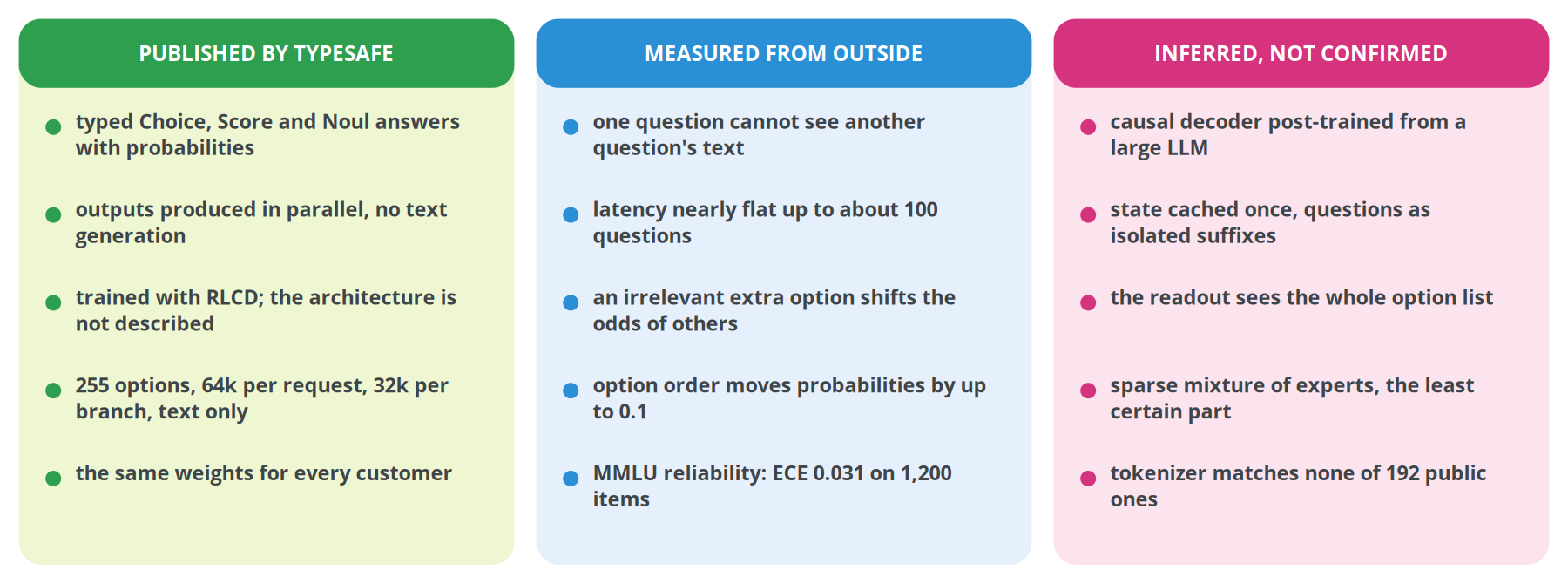
Search for how Jev works and you will find confident answers. It is a diffusion model; it is a BERT; it is GPT with constrained decoding; it is a mixture of experts. TypeSafe has confirmed none of them.
With the concepts of Chapters 4 to 9 in place, the evidence about Jev can be read precisely. This chapter sorts it into the three kinds introduced at the start of the book.
What TypeSafe states
published TypeSafe AI released Jev in early access on 15 September 2026 [1]. Its founder, Diogo Almeida, is a co-author of the InstructGPT paper behind ChatGPT's post-training [1][40]. The launch post describes a new stack with three parts: a new model architecture, a parallel sampler and a training method called RLCD. The architecture itself is not described [1].
published The current model is jev-1.13.0. It reads text only, is trained mainly on English, serves the same weights to every customer and is not trained on customer requests [6].
published TypeSafe claims 70 to 500 ms per request, and speedups of 193.6 times and cost reductions of 444.6 times over frontier language models on four published workflow evaluations. In those evaluations the reference answers are the average predictions of two frontier models, and TypeSafe describes the speedups as the high end of what to expect [1].
TypeSafe also publishes a page of known weaknesses of Jev 1.13, discussed in Chapter 13 [7].
RLCD as described
published TypeSafe's primer places RLCD beside two familiar post-training methods [5]. RLHF turned pretrained models into chat assistants by rewarding responses people prefer. RLVR produced reasoning models by rewarding answers that can be checked automatically. RLCD trains a model to return decisions and probabilities, with the target that a higher probability should mean a higher chance of being correct. The primer argues that preference training rewards sycophancy and confident-sounding answers, and that it narrows the model's output distribution, an effect it calls mode dropping [5].
inferred Nothing else about RLCD is public: not the loss, the reward, the data, or whether the method is reinforcement learning in the narrow algorithmic sense. A strictly proper scoring rule, as in Chapter 8, is the natural objective for the stated goal [9][34].
What the experiments show
Hume's essay of 17 September is the most careful outside study. It reports about 10,000 API calls, publishes every request and response, and states which conclusion rests on which experiment [9]. The measurements below come from it, and each one tests a property introduced earlier in this book.
measured Questions are isolated, as in Chapter 6. A secret code placed in one question was reported with probability 0.00 by another question, the same as when the first question was removed. With the code in the state, the probability was 0.90 to 0.92.
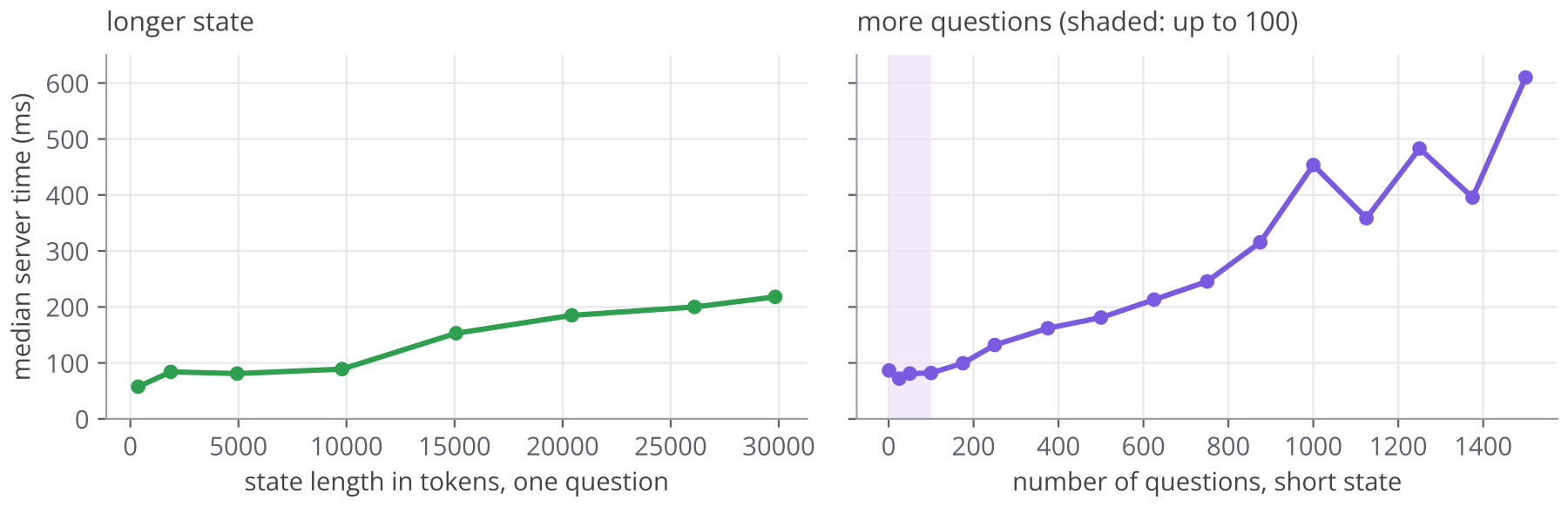
measured The state is processed once. Server time barely changed as the number of questions grew to about 100, and then grew slowly; 1,500 questions on a short state still returned within a few hundred milliseconds. Per token, question text cost about twice as much server time as state text. A request with a 23,000-token state and 5,000 questions was accepted, which is possible only if the state counts once against the 64,000-token request limit.
measured The API's output_tokens field is a billing figure. Its value depends on the question identifiers, which never reach the model, so it is computed from the serialized response after inference and does not count generated tokens.
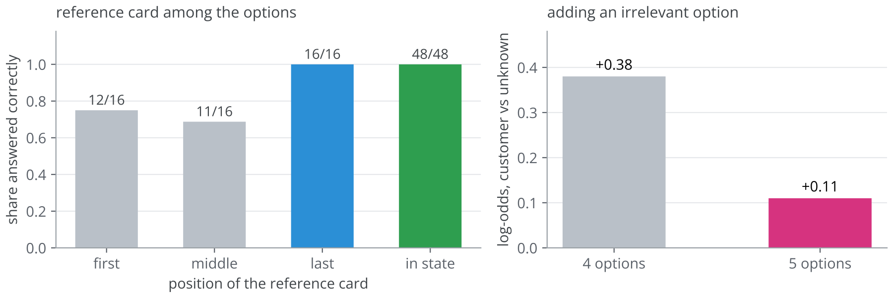
measured Options influence each other, as in the listwise designs of Chapter 5. Appending an irrelevant fifth option shifted the log-odds between two existing options from +0.38 to +0.11, averaged over ten randomized blocks. If each option had a fixed score and one softmax were applied, those odds could not change. A reference card placed as the last option was read correctly in 16 of 16 trials, and in 12 and 11 of 16 when placed first or in the middle. Reversing the order of options moved one support classification from 0.84 to 0.89 up to 0.93 to 0.96.
measured On a 1,200-question MMLU sample the ECE was 0.031, with most answers in the top probability bin, as Chapter 7 discussed. MMLU-Pro accuracy was 84.6%.
measured Jev's token counts matched none of 192 public tokenizers across 415 probes; the closest, Qwen's, agreed on 348.
The most likely reconstruction
inferred From these results Hume proposes a causal transformer post-trained from a large pretrained language model, with the state encoded once as a shared prefix, each question as an isolated branch, a readout that sees the full option list, and heads trained on distributions [9]. He argues for a decoder backbone because this breadth of knowledge comes from large-scale pretraining and every model at that scale is a causal decoder, and he notes that his experiments cannot tell a decoder from an encoder. He expects a sparse mixture of experts and marks it as the least certain part.
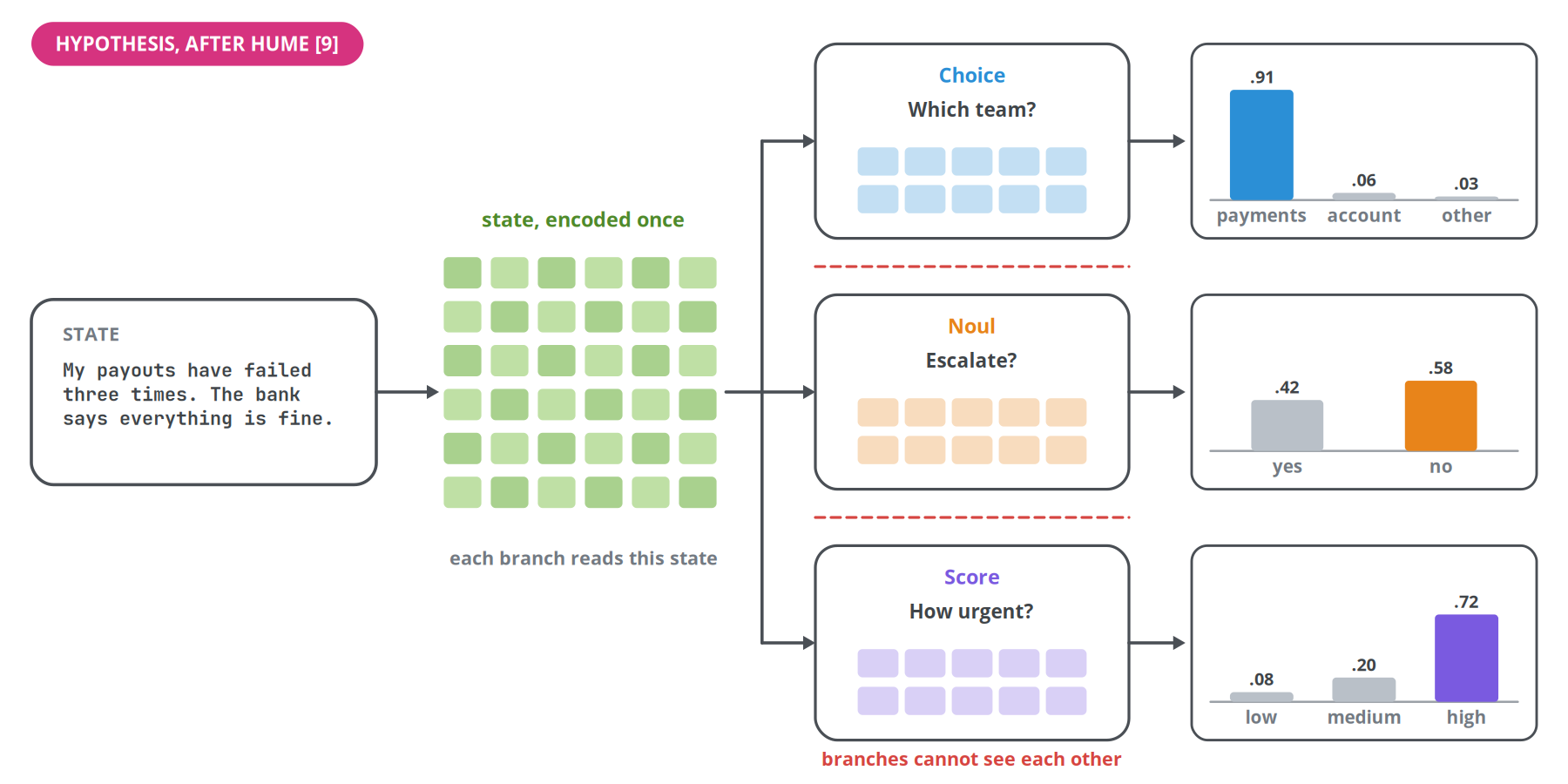
Kev's block-causal mask and pointer head from Chapters 5 and 6 implement this reconstruction directly [10]. When you read a claim about Jev's internals, check whether the author separates measurement from inference. Secondary coverage often does not: zephel01 found that Latent Space's roundup of the first reproductions linked its SemIf section to a different person's model, and that the wrong link spread to other articles [25].
Chapter 11
The open models
Ten days after Jev's launch, a tracker on Hugging Face listed 50 open entrants [22]. Each one is a choice of readout from Chapters 4 and 5, a training recipe from Chapter 8 and a dataset from Chapter 9.
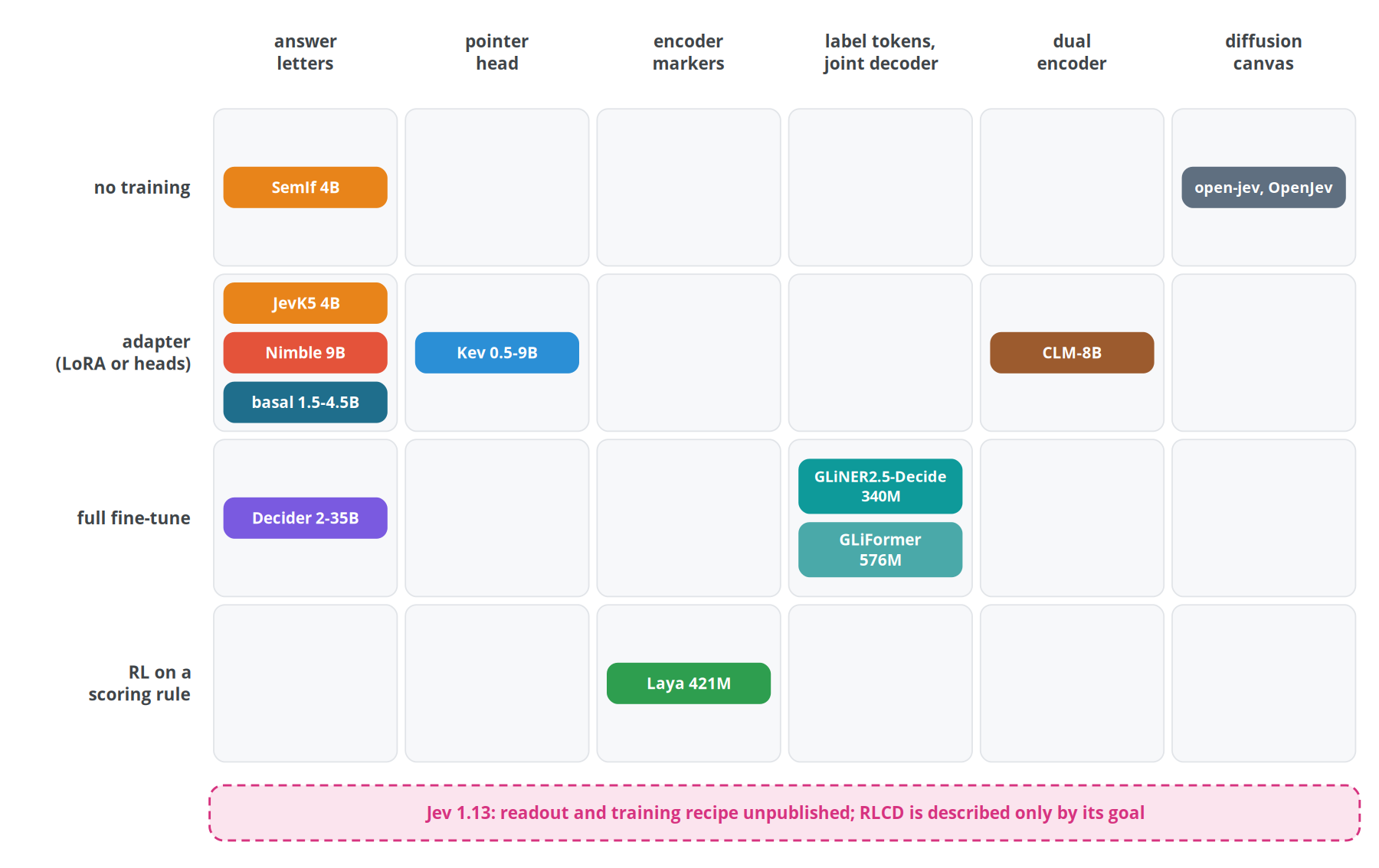
| Model | Base network | Size | Readout | Training | Licence |
|---|---|---|---|---|---|
| Kev [10] | Qwen2.5, later Qwen3.5 | 0.5B to 9B | pointer head | LoRA and head, cross-entropy | Apache 2.0 |
| SemIf [11] | Qwen3.5-4B, frozen | 4B | answer letters | none | MIT (code) |
| JevK5 [12] | Qwen3.5-4B | 4B | answer letters, T = 1.532 | LoRA, distilled from a 27B teacher | Apache 2.0 |
| Bespoke Nimble [13] | Qwen3.5-9B | 9B | one-token answer codes | LoRA on contrastive pairs | see repository |
| Decider [14] | Qwen3.5 2B, 4B and 35B-A3B | 2B to 35B | letter rows at answer slots | all weights, 742M tokens | Apache 2.0 |
| AutoJev-27B [20] | Qwen3.8-27B | 27B | probabilities over options | all weights, 73,000 examples | Apache 2.0 |
| Laya [15] | ModernBERT-large | 421M | mask tokens and a head | RL on scoring rules | Apache 2.0 |
| GLiNER2.5-Decide [16] | DeBERTa-v3-large | 340M | label tokens, joint decoder | fine-tune of GLiNER2 | Apache 2.0 |
| GLiFormer [17] | DeBERTa | 576M | task heads | multitask supervised | Apache 2.0 |
| CLM-8B [18] | Qwen3-8B, frozen | 8B and two heads | dot product | InfoNCE in three stages | Apache 2.0 |
| open-jev [19] | DiffusionGemma 26B-A4B | 26B, 3.8B active | canvas logits | none | MIT (code) |
| basal-1.0 [52] | Bielik v3, Polish | 1.5B and 4.5B | answer letters, two orders averaged | LoRA (4.5B), distilled full fine-tune (1.5B) | Apache 2.0 |
| MedDecider | Qwen3.5, Qwen3.8, Gemma 4 | 4B to 31B | answer letters, two orders averaged | LoRA, medical decisions | CC BY-NC 4.0 |
The profiles below add what the table cannot: how each project was built and what its authors say it gets wrong.
Kev
Jared Palmer built the first Kev, kev-0.5b, as a laptop-scale test of Hume's reconstruction: a LoRA adapter and a pointer head on Qwen2.5-0.5B, trained in about 1 hour 45 minutes on an Apple M5 on six public datasets [10]. It is the clearest reference implementation of question isolation. The later family on Qwen3.5 comes in 0.8B, 4B and 9B sizes. The authors say they do not know Jev's training data, so they do not treat their comparisons with Jev as controlled.
SemIf and JevK5
SemIf, by Theo Lee, reads answer letters from a frozen Qwen3.5-4B and runs in a browser through WebGPU as well as on a single consumer GPU [11]. It was called OpenJev until its author renamed it. On 102 public evaluation rows that TypeSafe released, its answers matched the reference distribution's top choice 0.845 of the time, against 0.883 for Jev's published answers; SemIf did not call the live Jev API.
JevK5, by Alibi Serikbay, keeps SemIf's prompt and readout and adds the distillation recipe of Chapter 8 [12]. On JevBench v1.4, which combines accuracy, calibration, speed and cost, it scored 62.04 against Jev's 63.29 and ranked second of 76 systems. On 308 new sealed questions its accuracy was 33.1% against Jev's 36.7%, and on 231 public questions 85.3% against 86.6% [12][23].
Bespoke Nimble
Bespoke Labs built Nimble in one day, by its own account, and published the recipe together with the checkpoint [13]. A rank-16 LoRA on Qwen3.5-9B is trained for one epoch on 2,676 contrastive examples. The team did not distil from Jev. On its 324 held-out examples, Nimble matched 90.1% of the reference labels, against 66.4% for the untuned base model, 84.9% for an untuned 27B model and 93.2% for Jev 1.13. The held-out set comes from six source families, and the team calls it a narrow test.
Decider, AutoJev and the Decision 1.0 family
Decider trains every weight of Qwen3.5-4B-Base on 1.89 million items and 742 million tokens, then refines it with a rank-64 LoRA on 29,325 harder rows [14]. There is no reinforcement learning stage. A 35B mixture-of-experts version also exists.
AutoJev-27B was built largely by autonomous agents, from data generation to deployment, with a full fine-tune of Qwen3.8-27B on 73,000 examples on one H200 GPU [20]. It reports 84.6% accuracy against 82.8% for Jev on its own benchmark self reported, and it is the highest-scoring open entrant on the independent Decision Index 0.2, at 50.9 against Jev's 51.7 [22].
The Decision 1.0 family from the semantic-router community ships checkpoints from 0.6B to 9B, both encoders and decoders. Its 9B model reports 77.4% on a 54-task benchmark; the authors state that the category weights were chosen after they saw the results [21].
Laya
Laya is the encoder design of Chapter 5, trained with its own version of RLCD [15]. A 322M multilingual variant built on mmBERT covers more than 100 languages, and a router picks the checkpoint by detecting the script of the input. The model card lists its limits: base checkpoints near chance on the typed-decisions benchmark before fine-tuning, a collapse on option lists longer than the budget allows, and an act head that does not work yet. zephel01 also noticed that Laya's README and its model card report two different sets of numbers, so a quoted Laya result should name its source [25].
GLiNER2.5-Decide and GLiFormer
GLiNER2.5-Decide adds joint decoding under rules to the GLiNER2 extraction model [16][28]. On Fastino's Fast Decisions benchmark, 17 operational domains with 300 held-out examples each, it led 9 of 17 datasets with an average of 60.1% self reported, including 75.3% on support intent. The weights run on a CPU and a 1B version also exists.
GLiFormer from Knowledgator is a 576M encoder with heads for named entities, classification, relations, nested records and embeddings [17]. It is mainly an extraction model that can also answer Choice-shaped questions.
CLM-8B
CLM-8B is the dual encoder of Chapter 5 [18]. Fine-tuned as a verifier that picks the best of several candidate solutions from a coding agent, it reports 81.6% on DeepSWE and 87.6% on Terminal-Bench 2.1 self reported. The team has announced a multimodal CLM-35B for early October 2026.
DiffusionGemma harnesses
Two projects read decisions from DiffusionGemma without training [19]. The open-jev harness by JoshuaSP is an inference script; zephel01 reports that on a 337-question evaluation it matched 86.1% of saved Jev answers with one denoising step and 87.8% with two, against Jev's 90.8% agreement with the references [25]. OpenJev by razorback16 packages the same idea as a server with the TypeSafe API and needs a GPU with at least 24 GB of memory. On the Decision Index, the untrained harness scored 44.2, above most fine-tuned 4B and 9B decoders [22]. That result suggests the base model's knowledge matters more than the readout.
Liquid d1
Liquid AI released d1 at the end of September as a hosted model behind its own API, and added image input on 5 October [67]. Like Jev, it reads the state and the questions in one forward pass and returns probabilities without generating tokens, with the same Noul, Choice and Score question types. Liquid bills only input tokens, at $0.04 per million, and quotes 200 to 300 ms for a text decision through the API. The weights and the size of the hosted model are not published, and Liquid describes it as the first model to rival Jev on text decisions [67] self reported.
On 7 October Liquid released two open-weight models [68]. d1-3B is trained from LFM2.5-VL-3B, a 3.1B decoder that reads images as well as text. d1-omni-600M starts from LFM2.5-Encoder-350M, a bidirectional encoder, with image and audio encoders added, so it can take a voice recording as input without a transcription step; Liquid calls it an early research release. For Choice and Score questions d1-3B returns a probability for every option, and for a Noul question only the probability of yes. Its model card lists 16 languages, Polish among them. Both models use the LFM Open License v1.0, under which a company with annual revenue of $10 million or more needs a separate license for commercial use [69].
At release, Liquid reported 48.57 for d1-3B on Decision Index 0.2.1, ahead of every 4B and 9B entrant listed then and of the 35B Decider at 47.11 [68] self reported. One question takes 8 ms on an RTX 4090 and 50 ms on a Jetson Orin Nano, the slowest device Liquid measured. The lead did not last. On Decision Index 0.3.2 a week later, which adds private tests and counts unsupported requests as wrong, d1-3B had a full score of 38.9, against 55.8 for the best entrant under 10B and 60.1 for Jev 1.13 [70].
basal-1.0
basal-1.0, by Remigiusz Kinas, is a Polish decision model built on the Bielik v3 family. It uses the answer-letter design of Chapter 4 with both option orders averaged in one pass, and it is trained on data whose labels are mostly computed by code. On held-out Polish decisions the 4.5B model scores 0.884 against 0.780 for Jev. Chapter 14 describes it as a case study [52].
MedDecider
MedDecider, from TheLion.AI, applies Jev's contract to medicine: a clinical note, trial record or JSON state goes in with a question of 2 to 10 options, and a calibrated probability for each option comes out of one forward pass per option order. It comes as LoRA adapters on Qwen3.5-4B, Qwen3.5-9B, Qwen3.8-27B and gemma-4-31b-it, plus a Duo that averages the 31B and 27B. Against Jev 1.13, the 31B scores 70.2% against 65.4% on unseen medical exams, 88.8% against 79.5% on robustness tests, and follows an instruction planted in a note 2.7% of the time against 13.7% self reported. The adapters are under CC BY-NC 4.0, so commercial use is excluded, and the training notes are synthetic.
Chapter 12
Using decision models in production
A support team receives 40,000 tickets like the running example every day. Each needs a team, a priority, a check for legal threats and a decision on whether a refund can be issued without a person.
Code decides, the model judges
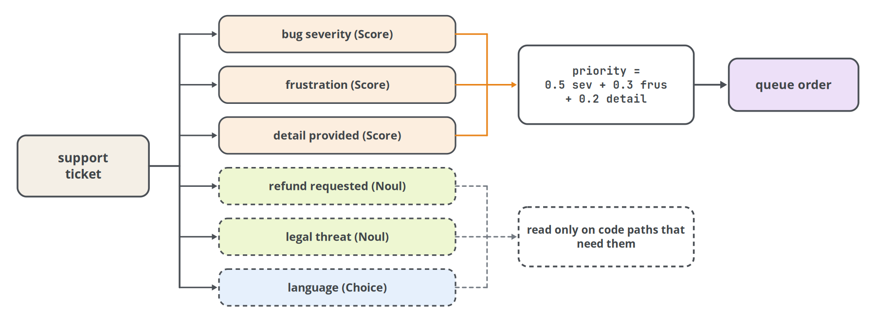
TypeSafe's design advice applies to every model in this book. Ordinary code owns the workflow, and the model is asked only for narrow judgments that code cannot compute [3]. A broad question such as "how important is this ticket?" becomes several simple questions whose answers the code combines with weights it controls. When priorities change, you change a weight in code, and the prompt stays the same. TypeSafe calls this composite scoring. Combined with speculative fan-out, which asks every question the code might need in one request and ignores the answers it does not use, a request for our ticket looks like this:
Acting on confidence
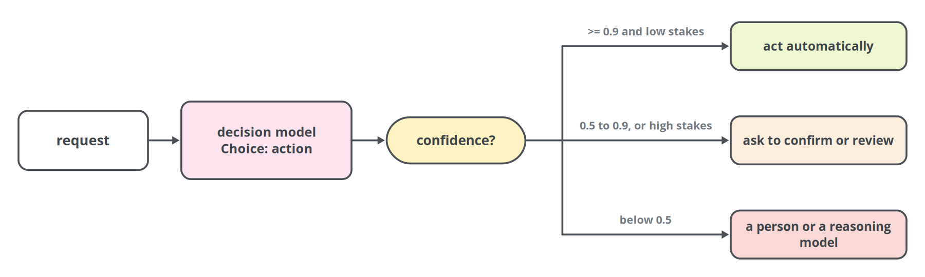
The answer says what the model thinks. The probabilities say whether to act on it. A common starting point is three bands: act automatically, ask for confirmation, and hand over to a person [4]. The thresholds belong to the action. Showing the customer a help article can run at a lower bar than issuing a refund.
from typesafe_sdk import Choice, TypeSafeClient

# The same code works against a local Kev, Laya or CLM server via base_url=...
client = TypeSafeClient(model="jev-1.13.0")        # pin the version
r = client.system_one(
    state=ticket_text,
    questions={"action": Choice(
        instructions="What is the customer asking us to do?",
        criteria={"refund": "Return money for a charge",
                  "rebook": "Replace a cancelled order",
                  "info": "Only asking for information",
                  "other": "None of the above"})})
a = r.answers["action"]
if a.confidence < 0.5:
    send_to_human(ticket_text)
elif a.choice == "refund" and a.confidence < 0.9:
    ask_customer_to_confirm()
else:
    run_workflow(a.choice)
Kev's README shows the official SDK running unchanged against its local server when base_url points to it [10].
Cascades
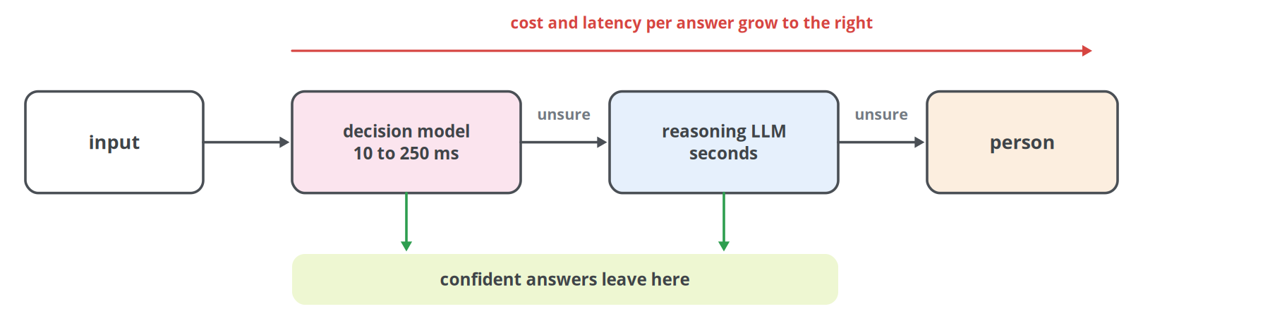
A decision model does not replace a reasoning model. It decides when one is needed. In a cascade the fast model answers first. Confident answers leave the pipeline at once, and uncertain ones go to a reasoning model and then to a person. TypeSafe's cookbook for structured extraction follows this shape, with a cheap first pass, a verification step, and a reasoning model only for what remains [8].
Patterns from the TypeSafe cookbooks
TypeSafe's documentation contains worked recipes that transfer to the open models [8]. In re-ranking, one Noul per pair of query and candidate over 30 keyword-search candidates raised top-1 accuracy on the CLERC legal retrieval set from 5% to 18%, and top-10 accuracy from 38% to 62%. For retrieval-augmented generation, a Noul per retrieved passage decides which passages reach the answering model, and a Choice checks whether a quoted source supports the claim it is attached to.
Extraction can be phrased as choice. A regular expression or a generative model proposes candidate values, and the decision model picks one; dates become Choices over day, month and year that code assembles and compares. Function calling maps function names and closed-set arguments to typed questions, and one cookbook ranks 182 agent skills and then re-checks the top three with fuller descriptions. For guardrails, every message into and out of an LLM application gets hazard Nouls and a severity Score; GLiNER2.5-Decide can also enforce that a detected harm implies an unsafe verdict [16].
Real-time control is possible at these latencies. TypeSafe's launch demos include a Doom bot making about ten queries per second, which costs roughly $7 per hour, and a Wikipedia navigation game with hundreds of links to choose from at each step [1]. For agents with a fixed set of actions, CLM's cached action embeddings were designed for this setting [18].
Chapter 13
Failure modes and security
Check Point gave an attacker control of one section of an investment report that described a textbook Ponzi scheme. For about fifty cents per attempt, the attacker made Jev rate the company low risk and recommend investing.
Known weaknesses
TypeSafe's list of Jev 1.13 weaknesses is a good checklist for any decision model [7]. The model reads instructions literally. It does not count reliably, it judges numbers better when they are written as words, and it compares dates poorly. Accuracy falls with multi-step indirection, with double negatives and with long stretches of irrelevant state. Adversarial content in the state can steer it. Contradictions between the instructions and the criteria confuse it. It is not trained to generate text. The remedy is the same in each case: keep arithmetic, dates and filtering in code, split compound judgments into separate questions, and send only the part of the state a question needs [7].
Question wording changes the answer
Relations between questions that seem obvious do not hold. On an ambiguous ticket, "Is the customer asking for a refund?" returned 0.22 as a Noul and put 0.01 on "yes" as a two-option Choice. On a ticket reading "I was charged twice for the same order. Can someone look into this?", the Noul "Is the customer asking for a refund?" and its negation "Is the customer asking for something other than a refund?" returned 0.72 and 0.47, which add up to 1.19 [7]. zephel01 found that the same judgment, asked as one four-way Choice, was right 48.3% of the time on his 120 generated scenarios, and 98.3% of the time when split into four separate Nouls [25].
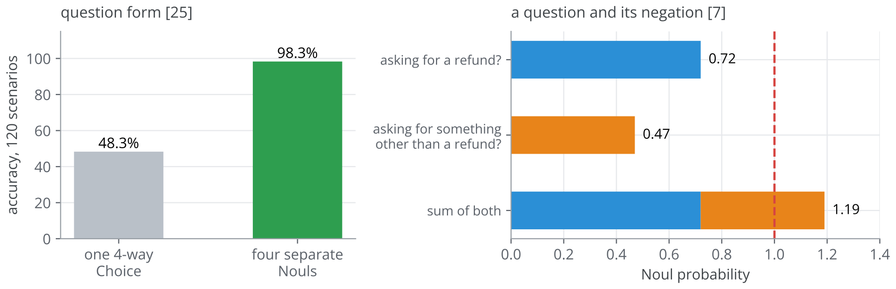
The documentation's advice follows: ask each decision in one form, word it to mean exactly what you want, and do not reuse a threshold tuned on a Noul for a Choice [7].
Option order
Readouts that place the options in the same sequence inherit the position biases that language models show on multiple-choice tests [38]. Kev's answers changed in 7.4% of cases across four option orders [10]. On Jev, reversing the options moved one probability by about 0.07, and a reference card placed first among the options was used correctly in 12 of 16 trials [9].
The fixes work at different stages. During training, Kev can penalize disagreement between two option orders [10]. At inference time, the open project ruling scores each question under several rotations of the option order and averages the log-probabilities [25]. During evaluation, a permutation test belongs in every test suite before a threshold near the decision boundary is trusted.
Prompt injection
Check Point tested Jev inside a realistic due-diligence assistant [26]. Without an attack, every model tested gave the correct verdict every time. With an attacker in control of one section of the uploaded report, every configuration broke at least once. The strongest attacker succeeded in 25 of 27 runs, on the fourth turn on average, at about $0.50 per success. The successful attacks gave the model no instructions. They added a believable appendix with a clean audit opinion and a revised risk table, and the model then judged the false evidence correctly.
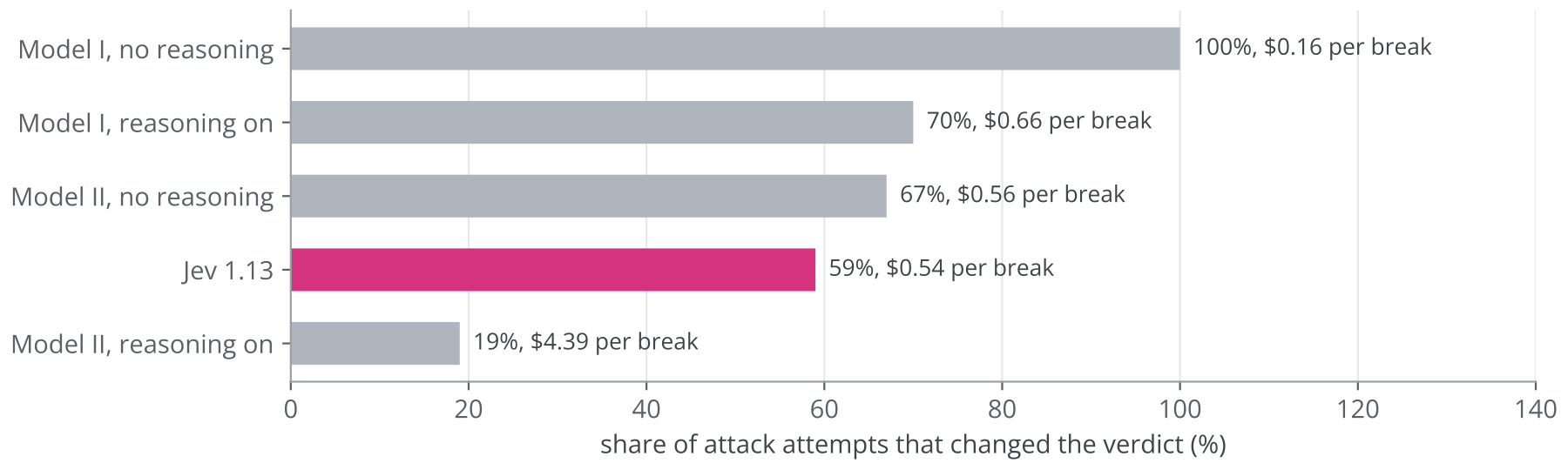
Delivering the document as a separate message marked as untrusted produced 16 breaks in 27 runs, the same as delivering it inline. An explicit instruction to ignore instructions inside documents changed the count from 18 to 17 of 27. The strongest defence measured was reasoning, which Jev does not offer: one language model with reasoning enabled fell to a 19% attack success rate at $4.39 per success [26].
A typed output limits what a model can say. It does not limit what the model can be persuaded to believe. Inputs need screening before they reach the decision; the decision should see as much genuine evidence as possible; irreversible actions belong behind higher thresholds or a person. Exposing probabilities to users also shows an attacker which way the model is leaning, since Check Point's attacker could see them. Indirect injection through retrieved content affects every application that feeds external text to a language model [48].
Distribution shift
A model calibrated on its training data can be confidently wrong elsewhere. Laya's English checkpoint reached 0.000 accuracy on Khmer text at 0.952 confidence [15]. Jev's documentation asks users to test non-English workloads before relying on them [6]. A new language, a new document type or a new customer segment is a new workflow and needs its own labelled check.
Chapter 14
Case study: basal-1.0, typed decisions in Polish
In September 2026 the best open 4B models lost 13 to 23 points of accuracy on Polish decisions compared with the English benchmark they were tuned for. basal-1.0, published by Remigiusz Kinas on 28 September 2026, was built to close that gap, and its report backs every design choice with an experiment [52].
Support ticketDzień dobry, za zamówienie A-104 pobrano ode mnie opłatę dwa razy. Proszę o zwrot duplikatu jeszcze dziś, inaczej zrezygnuję z abonamentu.
This chapter follows the report in the order the work was done. The case is useful beyond Polish for two reasons. Almost every concept of the earlier chapters appears in it, applied under one set of constraints. And the report publishes its negative results: distillation on generic text, early exits and a looped architecture were all measured and dropped.
Goals and the measuring stick
The project set five goals [52]. The model should be at least as accurate as Jev 1.13 on Polish decisions. Its probabilities should be trustworthy, measured as the share of decisions that can be accepted automatically while the error among them stays below 1% or 5%. It should give the same answer when the options are reordered. It should run locally and fast. And it should keep its English.
The second goal reflects the main finding of the baseline study. Jev's expected calibration error out of the box was 0.029, and the open models started far worse, but one temperature fitted on half of the data brought every open model to an ECE of about 0.05 or less [52]. A gap that one scalar closes is a poor target. Coverage at a fixed error budget, the number of decisions a team can actually automate, is harder to move, so the project competed on that.
What the baseline study found
Before training anything, the author built a frozen Polish development suite of 3,079 items in five tiers: Polish domain knowledge from professional exams, general knowledge in Polish, Polish decisions, Polish language understanding, and an English control. Jev and eleven open models from 1.5B to 12B parameters were evaluated with the same readout [52].
The gap to Jev was mostly knowledge. On Polish domain knowledge the best open models trailed Jev by 12 to 13 points. On Polish understanding and on synthetic decisions they came within 2 to 4 points, and the 11B Bielik model was statistically indistinguishable from Jev on both. That split shaped the project. Decisions can be trained; knowledge needs a larger model or has to be supplied in the state.
Choosing a base model and a tokenizer
The base is the Bielik v3 family of Polish models, whose 1.5B, 4.5B and 11B sizes share one 32,000-token Polish tokenizer called APT4 [52]. Chapter 6 explains why the tokenizer sets the cost of a decision. On identical Polish decision prompts, the tokenizers of Qwen3.5, Gemma 4, Llama 3.1, Mistral-Nemo and LFM2.5 needed 17% to 51% more tokens than APT4, and at a server batch size of 32 the same 4.5B network would make 15% to 34% fewer decisions per second with them. Multilingual vocabularies of 125,000 to 262,000 tokens did not close the gap. The small vocabulary also keeps the embedding and output matrices at 131 million parameters, where a 248,000-token vocabulary at the same width would need about one billion. English pays the price: APT4 needs about 1.6 times as many tokens on English prompts.
The shared tokenizer had a second benefit. A teacher and a student with the same vocabulary produce distributions over the same tokens, so the distillation of Chapter 8 is exact between them.
A faster base was tested and rejected. LFM2.5-8B-A1B is a mixture-of-experts model with about one billion active parameters per token. Its Polish was weak, 0.362 on Polish knowledge against 0.550 for Bielik-4.5B, and without training it chose by position and ignored the option text, changing its answer in 74% of questions when the options were reversed. The decisive problem was numerical. In bf16 the probabilities for one prompt changed by up to 0.37 with the other prompts in the batch, because rounding noise changed which experts the router selected, the mechanism described in Chapter 6. Keeping the router in fp32 removed the speed advantage that had motivated the choice [52].
Architecture: an ordinary decoder, read twice
basal-1.0 adds no new network. basal-1.0-4.5B is a 60-layer decoder with hidden size 2,048, SwiGLU feed-forward layers of width 11,008, grouped-query attention with 16 query heads and 2 key-value heads, RMSNorm, rotary positions, a 32,000-token context and an untied output head. It starts from the instruction-tuned Bielik-4.5B and is fine-tuned with a rank-32 LoRA on all linear layers, merged into the weights for release. basal-1.0-1.5B has the same design with 32 layers and hidden size 1,536 [52].
The readout is the answer-letter readout of Chapter 4 with two additions. The request is rendered in the chat template with options labelled A to J, and the assistant turn is prefilled with {"answer": ". The decision is the softmax over the logits of the allowed letters at that position. Every question is asked twice, in the original and in the reversed option order; the second distribution is mapped back to the original order and the two are averaged. A temperature fitted for each decision type is applied last. Both orders run in a single forward pass. The state and question are encoded once, and the two option blocks follow the shared prefix under a block mask that lets each block see the prefix and itself, the construction described for two orders in Chapter 6 [52].
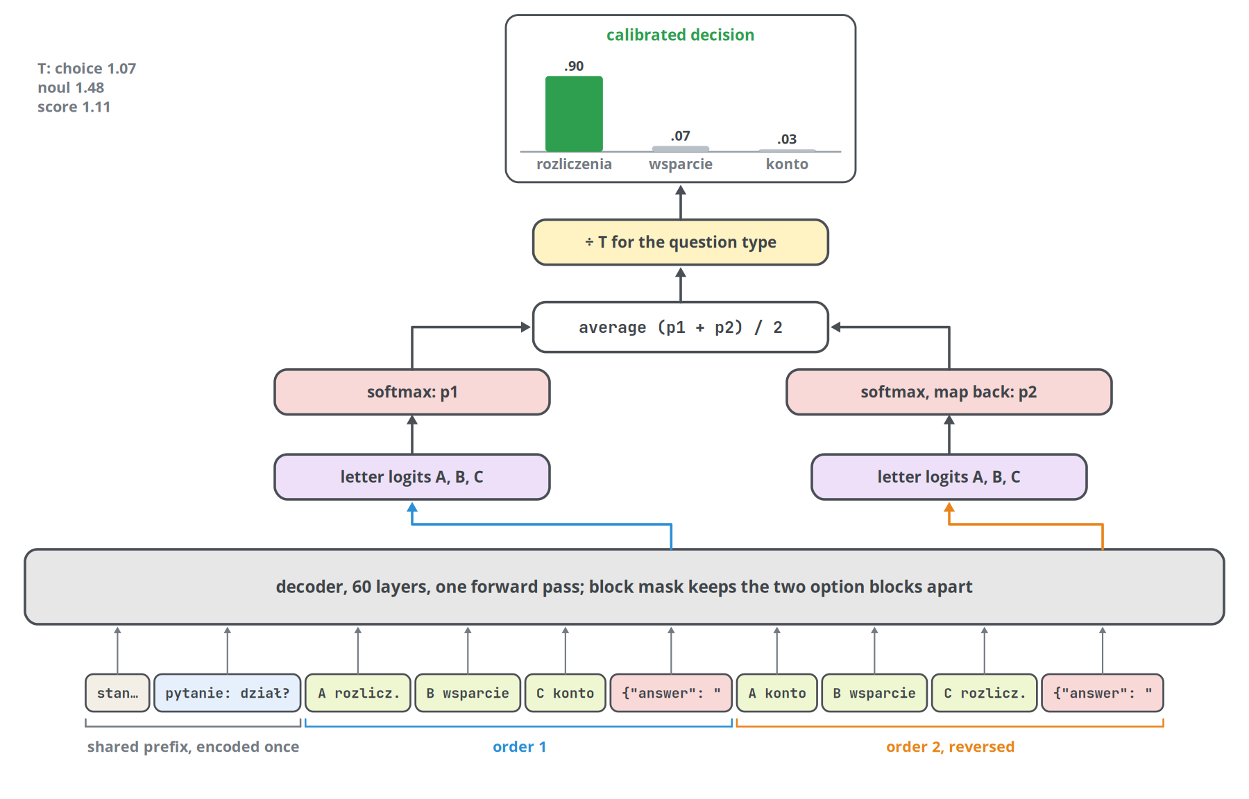
The fitted temperatures for the 4.5B model are 1.07 for Choice, 1.48 for Noul and 1.11 for Score. Asking in one order only costs 0.4 to 0.7 points of accuracy, and the top answer changes between the two orders on 5.8% of test items. Averaging an order with its reversal leaves the middle options in the middle, so the report claims reduced order sensitivity, not invariance [52].
Data: labels that can be audited
The training data is almost entirely synthetic, and every item records how its label was obtained. The report uses three sources, chosen so that no label rests on the opinion of one model [52].
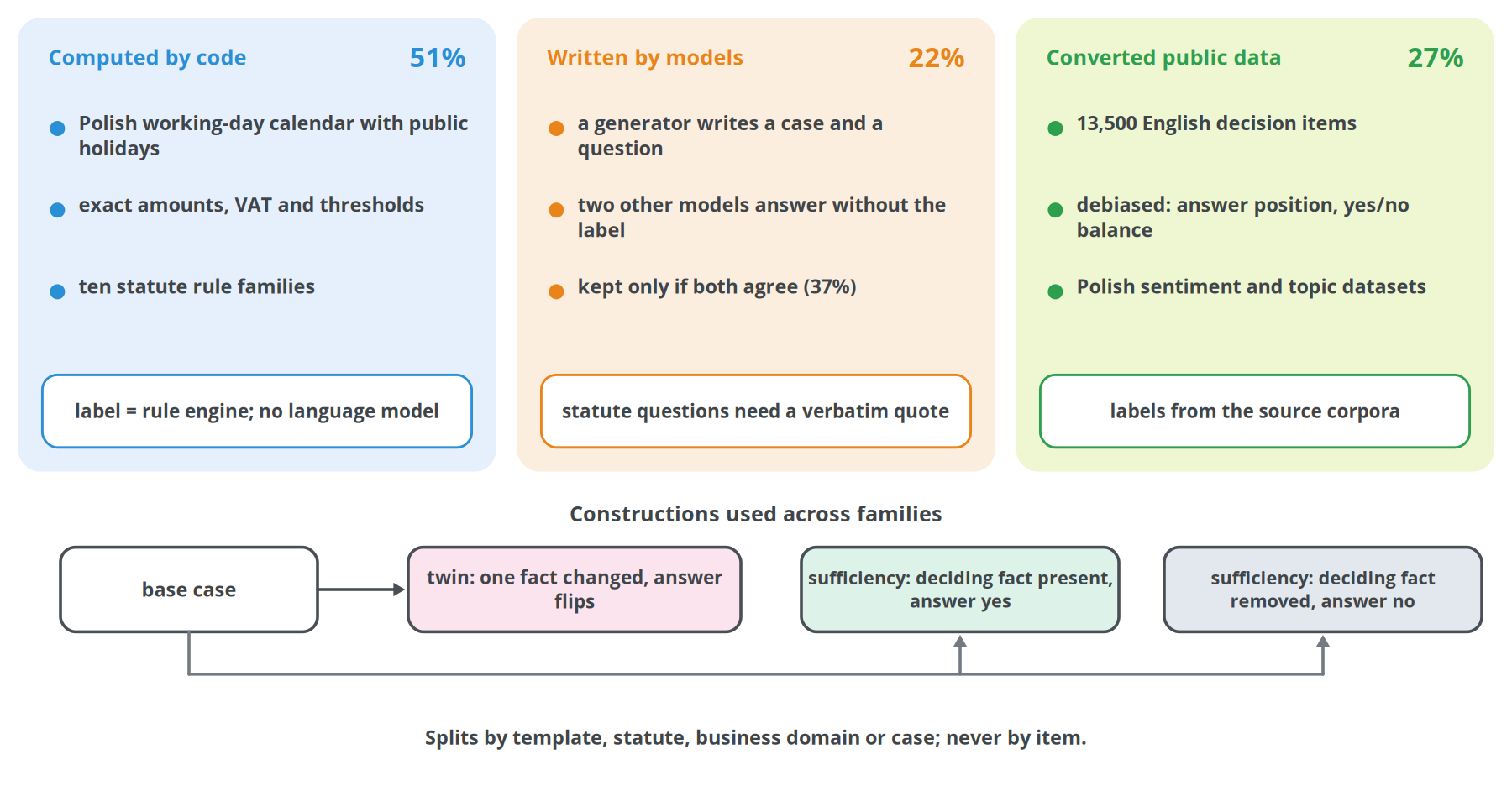
Items computed by code make up 51% of the training data of the released model. A Python generator draws the facts of a case, renders them into Polish or English text from hand-written templates and computes the answer with a rule engine: a Polish working-day calendar with public holidays for procedural deadlines, exact fractions for amounts and thresholds, and ten statute families covering labour-law notice periods and appeals, limitation periods, consumer withdrawal, statutory interest, court fees and personal income tax. Wrong options are the mistakes people make, such as a deadline that was not moved from a Saturday or a net amount where the gross was needed.
Items written by models make up 22%. For open-ended business decisions such as complaint handling, routing or urgency in fourteen domains, a generator model writes a case and a question, and two other models answer it without seeing the intended label. The item is kept only when both agree; 5,613 of 15,000 generated cases (37%) passed. Questions about statute text are generated from the passage itself and kept only with a verbatim quote as evidence.
Converted public data makes up 27%: 13,500 English decision items from a public typed-decision corpus, and two human-annotated Polish datasets for review sentiment and topic. The English corpus needed debiasing first. In the original, the correct option was listed first in 39% to 65% of questions and 70% of yes/no labels were "no", shortcuts a model learns at once.
Two constructions from Chapter 8 do much of the work. Rule families are generated as twins: the second item changes one fact or one rule so that the answer changes, and pairs that do not flip are discarded. Evidence-sufficiency pairs ask whether the state allows a decision at all, once with the deciding fact present and once with it removed. On those pairs the 4.5B model reached 0.95 to 0.96 where Jev reached 0.82, because Jev too often said the material was sufficient [52].
Splits are made by template, statute, business domain or case, never by item, so test items come from templates and domains that training never saw. A post-release audit recomputed every statutory family against the statutes in force and found one wrong rule: the notice-period generator ignored seniority reached during the notice period, which mislabelled 125 items. The evaluation labels were corrected. The released checkpoints were trained on the old labels and reproduce the error [52].
Training, one data version at a time
The data grew in four versions, and each one answered a weakness that the previous one had exposed.
With data v1, about 15,000 examples of deadlines, amounts and statute questions, one epoch of LoRA training with cross-entropy restricted to the option letters lifted the 4.5B model from 0.476 to about 0.83 on held-out templates, against 0.686 for Jev. Shuffling the option order in training cut the flip rate from 0.164 to 0.031 at equal accuracy. A Jensen-Shannon consistency penalty between two orders added nothing and was dropped. Decisions of types absent from the training data did not improve, which pointed at breadth as the next need [52].
Data v2 added twelve broad decision types and the evidence-sufficiency pairs, for 31,653 training items, and several ablations ran on it. A learning rate of 10-4, stable on v1, diverged on v2, and 5 × 10⁻⁵ was stable. A pointer head of the kind described in Chapter 5, scoring each option in its own segment, was perfectly order-invariant and less accurate (0.860 against 0.876). It also could not compare options: on choosing the last day among candidate dates it fell to 0.144, because each option saw only itself. Full fine-tuning of the pretrained base was worse than LoRA on the instruction model (0.823). The same recipe on the 11B model gained 2.7 points [52].
Data v3 added the English items. Polish accuracy did not fall, and the 4.5B model slightly passed Jev on English decisions. This version also tested distillation of the 11B model's option distribution, described in Chapter 8. It helped where the teacher was strong, raising a last-day date primitive from 0.739 to 0.838, and it hurt English, on which the teacher had never been trained. The rule that followed was to distil only from a teacher that is strong in the domain, and only on items where its top answer is correct [52].
Data v4 added the ten statute families built as twins and targeted items for formats that had regressed, for 63,663 training and 8,560 test items. On the new families the 4.5B model reached 0.921 against 0.635 for Jev. The distilled variant was not selected: on the calibration split it scored 0.844 against 0.847 for the plain cross-entropy model, and the test split was not used for the choice [52].
One family resisted every run: "was the filing on time?". The state does not give the length of the period, so a single forward pass has to recall the rule, count days with the holiday shift and apply the rule for the way the letter was sent. The fix was the composite-question advice of Chapter 12. Two elementary questions, "what is the last day of the period?" and "what is the legal filing date?", are asked about the same state and compared in code.
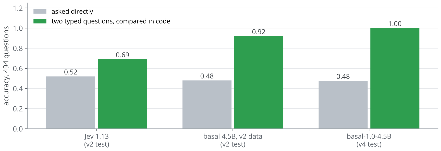
Asked directly, the released model answers "not on time" almost always and scores 0.476. Decomposed, it scores 1.000. Jev gains too, from 0.52 to 0.69, but less, because its date arithmetic is weaker [52].
The report also records an approach that failed early. Distilling Bielik-PL-11B's full output distribution into the 4.5B model on 50 million tokens of Polish web text lowered Polish knowledge by 2 points and left decisions unchanged. Its apparent calibration gain matched what one temperature achieves on the untouched model, so the run was stopped [52].
Calibration and selective automation
The released version was chosen on the calibration split. Temperatures and confidence thresholds were then fitted on exactly the predictor the server runs, one order-averaged distribution per item, and the thresholds for 1% and 5% accepted error were frozen before the test split was scored, the protocol described in Chapter 7 [52].
| System | Accuracy | ECE | Coverage at 1% target (observed error) | Coverage at 5% target (observed error) |
|---|---|---|---|---|
| basal-1.0-4.5B | 0.858 | 0.010 | 58.6% (1.22%) | 75.0% (4.41%) |
| basal-1.0-1.5B | 0.829 | 0.004 | 49.5% (1.37%) | 68.6% (5.55%) |
| Jev 1.13.0 | 0.772 | 0.014 | 18.1% (0.26%) | 49.0% (4.00%) |
With the 1% threshold frozen in advance, the 4.5B model decides 58.6% of test decisions automatically, and the error observed among them is 1.2%, slightly above the target. Under the same procedure Jev's threshold accepts 18.1%. Jev's observed error at that point, 0.26%, is far below the target, so its threshold turned out conservative on the test data; read off the test curve afterwards, a 1% budget would have allowed Jev about 30% and basal about 56%. The report states one limit of these numbers openly. The v4 test split was consulted during development, so the results come from an adaptive process on held-out templates and not from a single untouched final evaluation [52].
Where the decision forms: logit lens and early exits
Chapter 4 describes how a decision can be read from earlier layers. basal applied the logit lens to 2,870 readouts across all 48 families of the test split. Up to layer 49 of 60 the intermediate decision is at chance, both before and after decision training. Agreement with the final layer passes 50% at layer 50, 90% at layer 54, and reaches 99% only at the last layer [52].
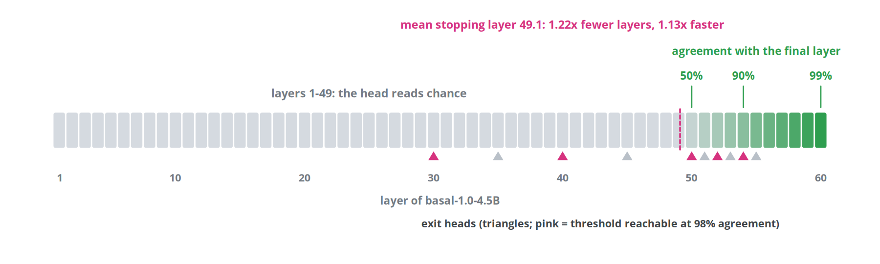
Trained exit heads, each an RMSNorm and a low-rank adapter in front of the frozen output head, were placed at layers 30 to 55. With a threshold per layer chosen on the calibration split for 98% agreement with the final layer, the forward pass stopped on average at layer 49.1. That is 1.22 times fewer layers, and single-request latency improved only 1.13 times. On the optimized serving path an agreement level of 0.99 takes a two-order decision from 12.2 to 10.5 ms. The target had been 1.5 times. Early exits ship as an optional setting per request and cost about 7 GB of extra memory [52].
Compression, introduced in Chapter 8, gave a similar picture. A 1.5B model of the same family, fully fine-tuned with decision distillation from the frozen 4.5B model for two epochs, lost 2.9 points for 2.5 times the throughput and half the memory, and was released as the lite variant. Pruning the 4.5B model to 36 layers lost 8.1 points, and pruning to 26 layers fell to 0.549. A looped model, with 48 middle layers replaced by one shared 16-layer block applied up to three times, did not train. Averaging the layers into one block destroyed the network, and decision data alone could not rebuild it [52].
Serving: from 177 ms to 12.5 ms
A decision is a prefill without generation, so its latency is the latency of one forward pass. At batch size 1, a 4.5B model on a 400-token prompt needs about 4 TFLOP, a few milliseconds of H100 compute, yet a plain bf16 PyTorch forward pass took 32 ms. The time went to launching thousands of small kernels. The project therefore optimized the serving path and checked after every step that decisions still agreed with the fp32 reference. Chapter 6 explains each technique [52].
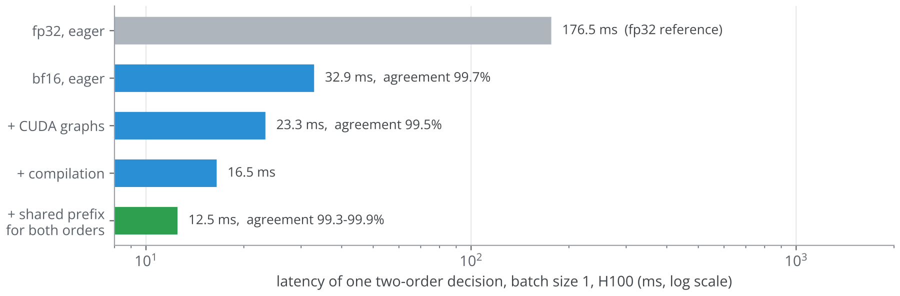
Moving from fp32 to bf16 took a two-order decision from 176.5 to 32.9 ms with 99.7% agreement. CUDA graphs brought it to 23.3 ms. Compiling the forward pass before capturing the graphs gave 16.5 ms. Packing both option orders after the shared prefix brought it to 12.5 ms, close to the 11.6 ms of a single order. Under load, batching by a token budget raised throughput from 25 to 63 two-order decisions per second on one H100 [52].
The fastest precision depends on the bottleneck of the machine. On a B300, bf16 is fastest at 8.8 ms, because a 4.5B model is limited by kernel launches there and quantization only adds work. On the H100, FP8 helps a little, from 12.5 to 11.3 ms. On an RTX PRO 6000 (18.9 to 14.9 ms) and an RTX 5090 (27.3 to 19.4 ms) it helps more. On a DGX Spark, which shares about 273 GB/s of memory bandwidth between CPU and GPU, FP8 halves the latency from 92.0 to 44.6 ms, because every forward pass at batch size 1 has to read all the weights. FP8 changes about 3% of decisions without lowering accuracy. 4-bit NVFP4 changes about 10% and costs about 3 points, so the report recommends it only for batched serving where throughput matters more than accuracy [52]. The 1.5B model needs 4.7 ms on a B300 and 7.7 ms end to end over HTTP on an H100.
Results against other systems
Every open system was served with its own official server on one H100 and queried through the same typed-decision interface by the same client, and every item was asked in both option orders [52].
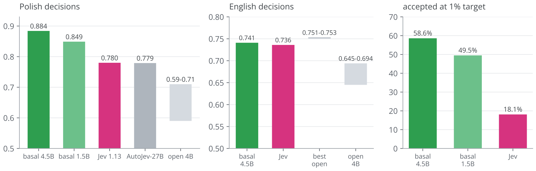
On Polish decisions the 4.5B model scores 0.884, against 0.780 for Jev and 0.779 for AutoJev-27B, the best open system; every open 4B system stays between 0.59 and 0.71. The test comes from basal's own generators, with unseen templates, so it favours basal, and the report says so. On English decisions basal scores 0.741 against 0.736 for Jev, a paired difference of +0.005 with a 95% interval from −0.020 to +0.029. The report calls this "not distinguishable", a weaker statement than "equal". On Polish general knowledge AutoJev-27B leads with 0.833 and basal scores 0.737, and on the public English JevBench items basal is last, at 0.74 against 0.76 to 0.88 for the open systems and 0.861 for Jev. The report presents the model as a Polish specialist [52].
Over HTTP, the released 4.5B engine answers in 13.9 ms and handles 57.4 decisions per second under 32 concurrent clients, both option orders included. The other systems' accuracies were measured with two requests per item, one per order, so a single request of theirs scores up to 3.2 points lower than the averaged figure. basal averages both orders inside one request [52].
Using basal-1.0
The engine implements the POST /v1/systemone interface, and its responses validate against the official schema. It supports Choice, Noul and Score questions with 2 to 10 options, since the readout uses the letters A to J. Several correct options are expressed as one Noul per option. A dependent question is asked speculatively alongside the question it depends on, as in Chapter 12. Amounts, dates and free text are out of scope unless the candidates can be listed as options. A request can set early_exit to off or to an agreement level, and "option_keys": "hide" reproduces the descriptions-only prompts on which the calibration was measured [52].
The report's moderation study uses the model as a classifier whose classes are written in the request. Each text is the state, and each moderation category is a Noul with a one-sentence Polish definition, along these lines:
{"state": "Tekst do oceny: ...",
 "questions": {
   "hate": {"type": "noul",
            "instructions": "Czy tekst obraża, poniża lub atakuje osoby albo grupy, np. ze względu na pochodzenie lub religię?"},
   "vulgar": {"type": "noul", "instructions": "..."},
   "selfharm": {"type": "noul", "instructions": "..."}}}
The model had no Polish moderation training and no examples in the prompt. On five Polish safety benchmarks it was significantly better than the Sójka-0.1B guard on four. Against the larger Sójka-0.5B, a classifier trained for exactly these categories, it was significantly better on two metrics, significantly worse on one and inconclusive on three. The fine-tuning data did contain 587 English moderation items, so the result is transfer from definitions, not moderation without any related training [52].
A taxonomy defined per request also answers questions that a fixed guard has no head for. On HateCheck-PL, asked which group a hateful text targets, as a Choice among seven groups and "none", the 4.5B model was right for 92.5% of 2,908 texts against a chance level of 12.5%, and it separated threats from other content with an AUROC of 0.913. A question about slurs showed the other side of the same property: the model answered the definition as written, and that definition also covered derogatory texts the benchmark did not label as slurs [52].
The cost is speed. Sójka-0.1B needs 4.2 ms per text and handles about 5,000 texts per second in batches; basal-4.5B needs 39 ms for five categories and handles 40 texts per second. Latency also grows with the number of questions, from 10 ms for one question to 100 ms for twelve, because the engine shares the prefix between the two option orders of one question and not between questions. The cross-question sharing of Chapter 6 would reduce this cost; the measured engine does not implement it [52].
Known limitations
The report lists its limitations, and anyone reusing the model should read them. Test items come from unseen templates but from the same generation pipelines as training, so claims about real Polish documents need a human-reviewed benchmark built from real cases, which the author names as the most important remaining step. Broad items kept by verifier agreement are easy by construction, and Jev scores 0.86 to 0.98 on them. Each variant is one training run with one seed. Polish world knowledge remains well below Jev's, 0.58 against 0.79. The released checkpoints reproduce the notice-period labelling error: for notice given within a month of three years of employment they answer one month where the law gives three. The quantized checkpoints inherit the bf16 calibration without validation, and the 13,500 converted English items could not be traced to their upstream sources [52].
What carries over to other languages
For a team building a decision model in another language, the report gives measured answers to several questions this book raised. A tokenizer and base model built for the language mattered more than any readout choice. Labels computed by code, twins and sufficiency pairs produced the largest gains, and the one rule error the audit found was learned exactly. One temperature fixed raw calibration, so the comparison that separated the systems was coverage at a frozen error budget. A composite rule split into typed questions went from chance to perfect. Most of the speed came from the serving path, and the architectural ideas for speed gave little or failed. The models, their FP8 and NVFP4 checkpoints, the engine and a scores-only Polish leaderboard are public under Apache 2.0 [53].
Chapter 15
Choosing a model
Leaderboards matter less for this choice than four facts about your deployment: whether the answer space is closed, where the data may go, whether you have labelled outcomes, and what hardware you have.
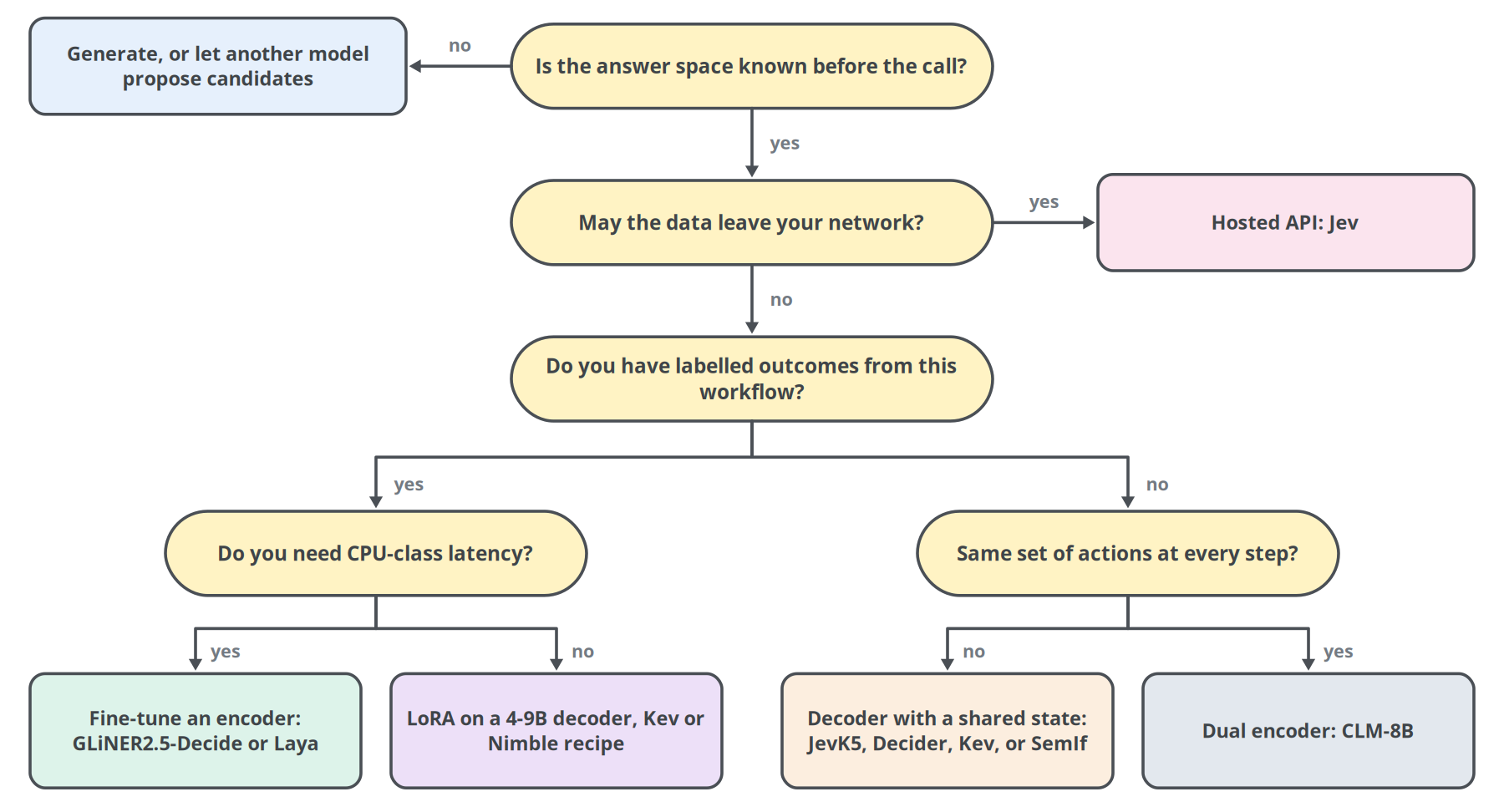
If the answer space is not known before the call, a decision model cannot help directly. Use generation, or a two-stage design in which something else proposes candidates and a decision model picks among them.
If the data may leave your network and the workload is in English, Jev requires the least work. It is well calibrated on public benchmarks, needs no GPU and costs cents per million tokens [6][9].
If the data must stay inside, the open models are credible, and labelled data from your own workflow decides between them. With labels, fine-tune. An encoder such as GLiNER2.5-Decide or Laya gives latency suited to a CPU, and a LoRA on a 4B to 9B decoder following Kev's or Nimble's recipe brings more general knowledge. Without labels, start with a large decoder that shares the state between questions, or with SemIf, which needs no training at all. If your agent scores the same set of actions at every step, CLM's dual encoder fits that shape [18].
If the decision has to run on a small device, or read an image or a voice recording, start with Liquid’s d1-3B or d1-omni-600M, and check the license before you build on them [68][69].
If the workload is not in English, check the tokenizer and the base model's knowledge of the language before anything else. For Polish, basal-1.0 is the measured option: it beats Jev on Polish decisions and answers in about 13 ms on one H100 [52].
Whichever model you choose, the work that decides success is the same. Pin the model version [6]. Collect labelled outcomes from your own workflow and fit a temperature on them. Set thresholds from the risk-coverage curve. Test option orders and alternative wordings of each question. Attack the inputs your application will read, the way Check Point attacked the due-diligence report, before a real attacker does.
References
- TypeSafe AI (D. Almeida). Introducing System One Models & Jev. Launch post, 15 Sep 2026. https://typesafe.ai/blog/introducing-system-one-models-and-jev
- TypeSafe AI. System One. Documentation, accessed 25 Sep 2026. https://docs.typesafe.ai/concepts/system-one
- TypeSafe AI. Primitives (Questions). Documentation. https://docs.typesafe.ai/primitives
- TypeSafe AI. Confidence. Documentation. https://docs.typesafe.ai/confidence
- TypeSafe AI. AI primer: RLHF, RLVR and RLCD. Documentation. https://docs.typesafe.ai/introduction/machine-learning-primer
- TypeSafe AI. Models: jev-1.13.0 limits, pricing, customisation, language support. Documentation. https://docs.typesafe.ai/models
- TypeSafe AI. Jev 1.13 jaggedness, last reviewed 17 Sep 2026. https://docs.typesafe.ai/model-jaggedness/jev-1.13
- TypeSafe AI. Documentation index with patterns and cookbooks. https://docs.typesafe.ai/llms.txt
- A. Hume. Jev's Architecture Unmasked. Essay with evidence bundle, 17 Sep 2026. https://archerhume.com/posts/jevs-architecture-unmasked
- J. Palmer. kev: a laptop-scale reconstruction of a Jev-style decision model. GitHub and model cards kev-0.5b, Kev-4B, Sep 2026. https://github.com/jaredpalmer/kev ; https://huggingface.co/jaredpalmer/kev-4b
- T. Lee. SemIf (formerly OpenJev): semantic ifs from open models. README and docs/METHOD.md, Sep 2026. https://github.com/TheoLeeCJ/SemIf
- A. Serikbay. JevK5 v0.2, open-weight Jev alternative. Model card, Sep 2026. https://huggingface.co/alibiserikbay/JevK5
- Bespoke Labs and M. Sathiamoorthy. Nimble: data, model and recipe for an open Jev. GitHub, Sep 2026. https://github.com/bespokelabsai/nimble
- Mapika. decider-4b: typed decisions with calibrated probabilities in one forward pass. Model card v2.1, Sep 2026. https://huggingface.co/Mapika/decider-4b
- Convai Innovations. Laya: multilingual, non-autoregressive System 1 decision model. Model card v0.3.20, Sep 2026. https://huggingface.co/convaiinnovations/laya
- M. Newhauser, Fastino Labs. GLiNER2.5-Decide: an open-weight model for structured decision making. Blog post and model card, 24 Sep 2026. https://fastino.ai/blog/gliner-2-5-decide-open-weight-decision-model ; https://huggingface.co/fastino/GLiNER2.5-Decide
- Knowledgator. GLiFormer Large v1. Model card. https://huggingface.co/knowledgator/gliformer-large-v1
- J. Kwok, H. Kang, T. Suresh, J. Saad-Falcon, M. Pavone, C. Ré, A. Mirhoseini. Contrastive Language Models: a System One model for fast and generalizable decision-making. Model card and repository, Sep 2026. https://huggingface.co/Contrastive-LM/CLM-v0.1-8B ; https://github.com/Contrastive-LM/CLM
- JoshuaSP. open-jev: typed JSON inference with DiffusionGemma; razorback16. OpenJev server. GitHub, Sep 2026. https://github.com/JoshuaSP/open-jev ; https://github.com/razorback16/openjev
- denis-pplx. AutoJev-27B. Model card, Sep 2026. https://huggingface.co/denis-pplx/autojev-27b
- llm-semantic-router. Decision-1.0-Lux-9B and the Decision 1.0 family. Model card, Sep 2026. https://huggingface.co/llm-semantic-router/Decision-1.0-Lux-9B
- multimodalart. Jev Reproductions Tracker, Decision Index 0.2 data (index.json), generated 25 Sep 2026. https://huggingface.co/spaces/multimodalart/jev-reproductions-tracker
- F. Standhartinger, Benchmark Heaven. JevBench. GitHub; the README marks results as preliminary. https://github.com/fstandhartinger/jevbench
- turlockmike. decide-lab: independent evaluation, calibration and LoRA fine-tuning of GLiNER2.5-Decide. GitHub, Sep 2026. https://github.com/turlockmike/decide-lab
- zephel01. I read 7 clones of Jev. Only the computational form was reproduced. note.com, 21 Sep 2026. https://note.com/zephel01/n/ne9a2c037e513
- Check Point. A decision model breaks like any other language model: a first look at Jev. 24 Sep 2026. https://blog.checkpoint.com/ai-security/jev-is-not-a-language-model-but-it-breaks-like-one-prompt-injection-against-a-typed-decision-model/
- Kotoba Labs. open-jev-deberta-v3-large. Model card, Sep 2026. https://huggingface.co/com-kotobalabs/open-jev-deberta-v3-large
- U. Zaratiana, G. Pasternak, O. Boyd, G. Hurn-Maloney, A. Lewis. GLiNER2: an efficient multi-task information extraction system with schema-driven interface. arXiv:2507.18546, 2025.
- U. Zaratiana, N. Tomeh, P. Holat, T. Charnois. GLiNER: generalist model for named entity recognition using bidirectional transformer. arXiv:2311.08526, 2023.
- T. Schick, H. Schütze. Exploiting cloze questions for few-shot text classification and natural language inference (PET). arXiv:2001.07676, 2020.
- Z. Zhao, E. Wallace, S. Feng, D. Klein, S. Singh. Calibrate before use: improving few-shot performance of language models. ICML 2021, arXiv:2102.09690.
- W. Yin, J. Hay, D. Roth. Benchmarking zero-shot text classification: datasets, evaluation and entailment approach. EMNLP 2019, arXiv:1909.00161.
- C. Guo, G. Pleiss, Y. Sun, K. Weinberger. On calibration of modern neural networks. ICML 2017, arXiv:1706.04599.
- T. Gneiting, A. Raftery. Strictly proper scoring rules, prediction, and estimation. Journal of the American Statistical Association 102(477), 2007.
- J. Juravsky et al. Hydragen: high-throughput LLM inference with shared prefixes. arXiv:2402.05099, 2024.
- J. Yao et al. DeFT: decoding with flash tree-attention for efficient tree-structured LLM inference. arXiv:2404.00242, 2024.
- R. Reddy et al. FIRST: faster improved listwise reranking with single token decoding. arXiv:2406.15657, 2024.
- C. Zheng, H. Zhou, F. Meng, J. Zhou, M. Huang. Large language models are not robust multiple choice selectors. ICLR 2024, arXiv:2309.03882.
- L. Tang, P. Laban, G. Durrett. MiniCheck: efficient fact-checking of LLMs on grounding documents. EMNLP 2024, arXiv:2404.10774.
- L. Ouyang et al. Training language models to follow instructions with human feedback (InstructGPT). arXiv:2203.02155, 2022.
- A. van den Oord, Y. Li, O. Vinyals. Representation learning with contrastive predictive coding (InfoNCE). arXiv:1807.03748, 2018.
- E. Hu et al. LoRA: low-rank adaptation of large language models. arXiv:2106.09685, 2021.
- D. Kahneman. Thinking, Fast and Slow. Farrar, Straus and Giroux, 2011.
- B. Warner et al. Smarter, better, faster, longer: a modern bidirectional encoder (ModernBERT). arXiv:2412.13663, 2024.
- P. He, J. Gao, W. Chen. DeBERTaV3: improving DeBERTa using ELECTRA-style pre-training with gradient-disentangled embedding sharing. arXiv:2111.09543, 2021.
- Z. Shao et al. DeepSeekMath: pushing the limits of mathematical reasoning (introduces GRPO). arXiv:2402.03300, 2024.
- OpenAI. GPT-4 technical report. arXiv:2303.08774, 2023. See the calibration plots before and after post-training.
- K. Greshake et al. Not what you've signed up for: compromising real-world LLM-integrated applications with indirect prompt injection. arXiv:2302.12173, 2023.
- DiffusionGemma Team, Google DeepMind. DiffusionGemma technical report. arXiv:2608.00146, 2026.
- Superpower Daily. Contrastive-LM releases an open model for faster agent decisions, with an accuracy tradeoff. 24 Sep 2026. https://superpowerdaily.com/posts/contrastive-lm-releases-an-open-agent-decision-model-that-runs-faster-than-jev-in-its-tests
- R. Williams. Simple statistical gradient-following algorithms for connectionist reinforcement learning (REINFORCE). Machine Learning 8, 1992.
- R. Kinas. basal-1.0: reliable, highly optimized typed decisions for Polish. Research report, version 1.0.1, Zenodo, 28 Sep 2026. https://doi.org/10.5281/zenodo.23022986
- R. Kinas. basal engine, models basal-1.0-4.5B and basal-1.0-1.5B, and the Polish typed-decision leaderboard. GitHub and Hugging Face, Oct 2026. https://github.com/rkinas/basal ; https://huggingface.co/spaces/Remek/jev-pl-benchmark
- G. Hinton, O. Vinyals, J. Dean. Distilling the knowledge in a neural network. arXiv:1503.02531, 2015.
- nostalgebraist. Interpreting GPT: the logit lens. LessWrong, 2020.
- N. Belrose et al. Eliciting latent predictions from transformers with the tuned lens. arXiv:2303.08112, 2023.
- T. Schuster et al. Confident adaptive language modeling. NeurIPS 2022, arXiv:2207.07061.
- A. Gromov et al. The unreasonable ineffectiveness of the deeper layers. arXiv:2403.17887, 2024.
- S. Bae et al. Relaxed recursive transformers: effective parameter sharing with layer-wise LoRA. arXiv:2410.20672, 2024.
- P. Micikevicius et al. FP8 formats for deep learning. arXiv:2209.05433, 2022.
- Y. Geifman, R. El-Yaniv. Selective classification for deep neural networks. NeurIPS 2017, arXiv:1705.08500.
- J. Devlin, M.-W. Chang, K. Lee, K. Toutanova. BERT: pre-training of deep bidirectional transformers for language understanding. NAACL 2019, arXiv:1810.04805.
- I. Loshchilov, F. Hutter. Decoupled weight decay regularization (AdamW). ICLR 2019, arXiv:1711.05101.
- C. Szegedy, V. Vanhoucke, S. Ioffe, J. Shlens, Z. Wojna. Rethinking the Inception architecture for computer vision (introduces label smoothing). CVPR 2016, arXiv:1512.00567.
- R. Müller, S. Kornblith, G. Hinton. When does label smoothing help? NeurIPS 2019, arXiv:1906.02629.
- M. Mosbach, M. Andriushchenko, D. Klakow. On the stability of fine-tuning BERT: misconceptions, explanations, and strong baselines. ICLR 2021, arXiv:2006.04884.
- Liquid AI. Introducing d1: the most capable decision model, now with vision. Blog, 5 Oct 2026. https://www.liquid.ai/blog/d1-decision-model
- Liquid AI. Multimodal open d1 decision models for the edge. Hugging Face blog, 7 Oct 2026. https://huggingface.co/blog/LiquidAI/open-d1
- Liquid AI. d1-3B and d1-omni-600M model cards, and LFM Open License v1.0. https://huggingface.co/LiquidAI/d1-3b ; https://huggingface.co/LiquidAI/d1-omni-600M
- multimodalart. Jev Reproductions Tracker, Decision Index 0.3.2 data (index.json), generated 15 Oct 2026. https://huggingface.co/spaces/multimodalart/jev-reproductions-tracker
Notes
- Qwen3.5 mixes full-attention layers with linear-attention layers [14], and a linear-attention layer cannot apply an arbitrary mask. Runtimes built on such models usually share the state through cache reuse: SemIf's shared mode prefills the state once and branches the questions, Nimble's Apple-silicon scorer processes the context once and scores all fields in parallel, and Nimble's CUDA scorer scores each field with the full prompt [11][13].